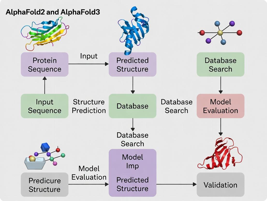
AlphaFold2 to AlphaFold3: A Comprehensive Guide to AI-Powered Protein Structure Prediction for Research & Drug Discovery
This article provides a detailed technical overview of DeepMind's AlphaFold2 and AlphaFold3 for researchers, scientists, and drug development professionals.
AlphaFold2 to AlphaFold3: A Comprehensive Guide to AI-Powered Protein Structure Prediction for Research & Drug Discovery
Abstract
This article provides a detailed technical overview of DeepMind's AlphaFold2 and AlphaFold3 for researchers, scientists, and drug development professionals. It covers the foundational principles of these revolutionary AI models, their methodological workflows and diverse applications, best practices for troubleshooting and interpreting results, and a critical validation and comparison of their accuracy, scope, and limitations. The goal is to equip practitioners with the knowledge to effectively leverage these tools for accelerating structural biology and therapeutic design.
Demystifying AlphaFold: The AI Revolution in Structural Biology from First Principles
Application Notes: The AlphaFold Revolution in Structural Biology
The development of AlphaFold2 (AF2) by DeepMind in 2020 and its successor, AlphaFold3 (AF3) by Google DeepMind/Isomorphic Labs in 2024, represents a paradigm shift in solving the protein folding problem. These AI systems have moved the field from a decades-long challenge of predicting protein structure from sequence to a new era of rapid, high-accuracy modeling, enabling novel applications in basic research and drug development.
Performance Benchmarks and Comparative Analysis
AlphaFold systems have been extensively benchmarked against traditional methods and experimental data.
Table 1: Comparative Performance of Protein Structure Prediction Methods (CASP Metrics)
| Method / System | Year | Global Distance Test (GDT_TS)* | Notable Capability |
|---|---|---|---|
| AlphaFold3 | 2024 | ~85-90 (est.) | Predicts protein complexes with ligands, nucleic acids, post-translational modifications. |
| AlphaFold2 | 2020 | 92.4 (CASP14) | High-accuracy single-chain protein structures. |
| AlphaFold1 | 2018 | 58.0 (CASP13) | Initial deep learning breakthrough. |
| Best Template Modeling | Pre-2018 | ~40-50 | Reliant on evolutionary homology. |
| Physical Simulation (Ab Initio) | - | Often <20 | Computationally intensive, low accuracy for large proteins. |
*GDT_TS: Metric from 0-100; higher scores indicate closer match to experimental structure. Scores for AF3 are estimates based on published data.
Table 2: Impact of AlphaFold Database (EMBL-EBI) as of 2024
| Metric | Value | Significance |
|---|---|---|
| Total Predicted Structures | >200 million | Vastly expands coverage of known protein space. |
| Coverage of UniProt | Nearly all cataloged sequences | Provides immediate structural hypotheses for most proteins. |
| Typical Model Confidence (pLDDT) | >70 for 58% of residues | Majority of predictions are usable for functional analysis. |
| Average Prediction Time | Minutes to hours per target | Drastic reduction from years of experimental work. |
Key Applications in Research and Drug Discovery
- Hypothesis Generation: AF2/3 models provide immediate structural context for site-directed mutagenesis, functional assays, and disease mechanism studies.
- Drug Target Assessment: Rapid evaluation of "druggability" by identifying binding pockets and analyzing surface features of novel targets.
- Complex Assembly Modeling: AF3 enables prediction of protein-protein, protein-nucleic acid, and protein-small molecule interactions, crucial for pathway analysis.
- Experimental Phasing: Predicted models serve as molecular replacement search models for X-ray crystallography, accelerating structure determination.
- Rational Design: Foundation for protein engineering, antibody design, and stabilizing mutations.
Experimental Protocols
Protocol: Utilizing AlphaFold2/3 forIn SilicoPoint Mutation Analysis
Purpose: To predict the structural and stability impact of a missense variant on a protein of interest.
Materials: See "Research Reagent Solutions" (Section 4.0).
Procedure:
- Sequence Retrieval & Preparation:
- Obtain the wild-type amino acid sequence (e.g., from UniProt:
P12345). - Generate the mutant sequence by introducing the specific point mutation (e.g., G12V) using a sequence editor.
- Obtain the wild-type amino acid sequence (e.g., from UniProt:
- Multiple Sequence Alignment (MSA) Generation (Optional for Local ColabFold):
- For AF2: Input the wild-type sequence into MMseqs2 (via ColabFold) or generate MSAs using tools like JackHMMER against a protein sequence database (e.g., UniRef30).
- For AF3 via Server: MSA generation is handled automatically.
- Model Generation:
- Option A (Cloud - AlphaFold Server): Submit wild-type and mutant sequences separately to the public AlphaFold server (if available for research use) or Isomorphic Labs' platform.
- Option B (Local/Colab - ColabFold): Use the ColabFold implementation (based on AF2) with default parameters. Run prediction for both sequences.
- Model Analysis:
- Download the predicted PDB files and per-residue confidence metrics (pLDDT or predicted aligned error).
- Load both structures into molecular visualization software (e.g., PyMOL, ChimeraX).
- Superimpose the mutant structure onto the wild-type structure using backbone atoms.
- Calculate the root-mean-square deviation (RMSD) of the local region (e.g., 5Å around the mutation site) and the global structure.
- Energetic Impact Prediction (Optional):
- Use tools like FoldX or RosettaDDGPrediction to calculate the predicted change in Gibbs free energy (ΔΔG) of folding upon mutation, using the AF2-generated structure as input.
- Interpretation:
- A high local RMSD (>1.5Å) and negative ΔΔG suggest a destabilizing mutation.
- Analyze changes in side-chain conformation, hydrogen bonding networks, or salt bridges.
Protocol: Using AlphaFold3 for Protein-Ligand Interaction Hypothesis Generation
Purpose: To predict the binding pose of a small molecule drug candidate within a protein target pocket.
Procedure:
- Input Preparation:
- Prepare the protein target amino acid sequence in FASTA format.
- Prepare the ligand molecule in SMILES string format or as a SDF/MOL file. Ensure correct protonation state.
- Submission to AlphaFold3:
- Access AF3 via the designated research interface (e.g., Google Cloud AlphaFold Notebook).
- Input the protein sequence and ligand definition into the appropriate fields.
- Define any known binding residues as optional constraints (if applicable).
- Submit the job for prediction.
- Output Retrieval and Validation:
- Download the resulting complex PDB file. The ligand should be included in the coordinates.
- Assess the model confidence scores provided for the ligand and binding site residues.
- Critical: Validate the predicted pose using complementary methods:
- Perform molecular docking of the same ligand into the same pocket using traditional docking software (e.g., AutoDock Vina, Glide) using the AF3 protein structure.
- Compare the AF3 pose with the top-scoring docking poses for consensus.
- Check for known pharmacophore features or key interactions from literature.
- Experimental Design Guidance:
- Use the predicted binding pose to design point mutations in the binding site for validation (see Protocol 2.1).
- Design focused compound libraries based on the predicted binding mode and fragment expansion.
Visualizations
AlphaFold3 Prediction & Application Workflow
Iterative AI-Experimental Research Cycle
The Scientist's Toolkit: Research Reagent Solutions
Table 3: Essential Resources for AlphaFold-Driven Research
| Item / Resource | Function / Purpose | Access / Example |
|---|---|---|
| AlphaFold Protein Structure Database | Repository of pre-computed AF2 predictions for nearly all known proteins. Serves as first-stop resource. | Publicly available via EMBL-EBI (https://alphafold.ebi.ac.uk) |
| AlphaFold3 Research Access | Platform to run AF3 predictions for novel complexes (protein, nucleic acid, ligand). | Google Cloud AlphaFold notebook or Isomorphic Labs partnership. |
| ColabFold | User-friendly, local or cloud-based implementation of AF2 and related tools. Enables batch runs and custom MSAs. | GitHub repository & Google Colab notebooks. |
| MMseqs2 (via ColabFold) | Ultra-fast search tool for generating multiple sequence alignments (MSAs), required input for AF2. | Integrated into ColabFold pipeline. |
| PyMOL or UCSF ChimeraX | Molecular visualization software. Critical for analyzing, comparing, and rendering predicted 3D structures. | Open-source (ChimeraX) or commercial (PyMOL) licenses. |
| FoldX Suite | Protein engineering tool for calculating stability changes (ΔΔG) upon mutation, using a PDB file as input. | Integrates with YASARA, PyMOL, or standalone. |
| RosettaDDGPrediction | Alternative, more advanced (but complex) suite for free energy calculation and protein design. | Requires license and computational expertise. |
| AutoDock Vina or Glide | Molecular docking software. Used to validate or compare AF3 ligand poses or for virtual screening on AF2 structures. | Open-source (Vina) or commercial (Glide, part of Schrödinger Suite). |
| UniProt Database | Comprehensive resource for protein sequences and functional annotation. Source of canonical sequences for prediction. | Publicly available (https://www.uniprot.org). |
| PDB (Protein Data Bank) | Repository of experimentally determined protein structures. Gold standard for validation of predictions. | Publicly available (https://www.rcsb.org). |
Application Notes
Within the broader thesis on the evolution from AlphaFold2 (AF2) to AlphaFold3 for protein structure prediction, the Evoformer module stands as the revolutionary core of AF2. It is a novel neural network architecture that jointly learns patterns from multiple sequence alignments (MSAs) and residue pair representations (templates and inferred potentials), enabling accurate, atomic-level structure prediction without reliance on known homolog structures.
Core Architectural Breakdown
AF2's architecture is a complex, recursive system that iteratively refines its predictions. The Evoformer is the heart of this refinement process.
Input Embeddings: The system ingests two primary data streams:
- MSA Representation: A tensor of size
(N_seq, N_res), whereN_seqis the number of sequences in the alignment andN_resis the number of residues. This captures evolutionary constraints. - Pair Representation: A tensor of size
(N_res, N_res). This encodes spatial and relationship information between residues from templates and other features.
- MSA Representation: A tensor of size
Evoformer Block Function: The Evoformer consists of a stack of 48 identical blocks. Each block performs communication between the MSA and pair representations via two core operations:
- MSA → Pair Communication: Updates the pair representation by considering interactions between all pairs of sequences in the MSA.
- Pair → MSA Communication: Updates each row and column in the MSA representation using information from the pair representation, effectively propagating spatial constraints back to the sequence data.
Output: After 48 blocks of iterative refinement, the final, information-rich pair representation is passed to the "Structure Module," which directly predicts the 3D coordinates of all atoms.
Table 1: AlphaFold2 Performance Metrics at CASP14
| Metric | Result | Significance |
|---|---|---|
| Global Distance Test (GDT_TS) | Median score of 92.4 on free modeling targets | Surpassed all other methods by a large margin; scores >90 are considered competitive with experimental accuracy. |
| Root-Mean-Square Deviation (RMSD) | Drastically reduced vs. next-best methods. | For many targets, predictions were within ~1 Å of the experimental structure. |
| Prediction Time | Order of minutes to hours per target (using TPUs). | Enabled high-throughput structural genomics applications. |
Table 2: Key Evoformer Hyperparameters from AF2
| Parameter | Value | Role |
|---|---|---|
| Number of Evoformer Blocks | 48 | Depth of the network; enables complex, iterative refinement. |
| MSA Representation Dimension | 768 | Channels for per-row (sequence) and per-column (residue) information. |
| Pair Representation Dimension | 128 | Channels for encoding relationships between each residue pair. |
| Attention Heads (MSA & Pair) | 8 (MSA row/col), 4 (Triangular) | Allows the model to focus on different types of dependencies simultaneously. |
Experimental Protocols
Protocol 1: Running AlphaFold2 forDe NovoProtein Structure Prediction
This protocol outlines the steps to generate a protein structure prediction using a standard AlphaFold2 implementation (e.g., via ColabFold).
I. Materials & Input Preparation
- Target Protein Sequence: Obtain the amino acid sequence (FASTA format) of the protein of interest.
- Computational Environment: Access to a high-performance computing cluster or cloud environment (e.g., with GPUs/TPUs). ColabFold provides a simplified, accessible interface.
- Databases: Download or have access to the required databases:
- UniRef90 (latest), BFD/MGnify: For MSA construction.
- PDB70 and PDB (mmCIF files): For template search.
- UniProt: (Optional) for full-sequence annotation.
II. Methodology
- Input Stage:
- Input the target FASTA sequence into the prediction pipeline.
- Feature Generation Stage:
- MSA Construction: Use HHblits (against UniRef90) and JackHMMER (against BFD/MGnify) to generate a deep multiple sequence alignment.
- Template Search: Use HHSearch against the PDB70 database to identify potential structural templates.
- Feature Processing: Compile MSAs, template features, and primary sequence features (e.g., predicted disorder, residue index) into the standardized input feature dictionary for AF2.
- Model Inference Stage:
- Load the pretrained AF2 model parameters (5 ensemble models).
- Pass the features through the AF2 neural network: a. The Evoformer stack (48 blocks) refines the MSA and pair representations. b. The Structure module (8 blocks) folds the refined pair representation into 3D atomic coordinates (including side chains).
- Run multiple random seeds (e.g., 25) per model to estimate prediction confidence.
- Output & Analysis Stage:
- Output Files: The run produces:
- Predicted structures in PDB format (ranked by confidence).
- Per-residue and per-pair confidence metrics: pLDDT (predicted Local Distance Difference Test) for model accuracy, and pAE (predicted Aligned Error) for relative positional confidence.
- Model Selection: Rank models by the average pLDDT score. The model with the highest score is typically the most reliable.
- Output Files: The run produces:
Protocol 2: Analyzing Evoformer Outputs for Interpretability
This protocol describes how to extract and visualize intermediate representations from the Evoformer to gain biological insights.
I. Materials
- A modified AF2 codebase that allows hooking into and extracting intermediate layer activations.
- Visualization libraries (Matplotlib, Seaborn, NGLview).
- The predicted structure and input features from Protocol 1.
II. Methodology
- Model Modification:
- Instrument the AF2 model code to save the activations from the MSA and pair representations at specific Evoformer block depths (e.g., blocks 1, 12, 24, 36, 48).
- Run Forward Pass with Tracking:
- Perform inference on the target protein while saving the specified intermediate tensors.
- Data Analysis:
- Pair Representation Analysis: Analyze the final pair representation (
(N_res, N_res, 128)) by reducing its dimensionality (e.g., via PCA) and plotting as a contact map. Compare this to the predicted pAE and the final 3D structure's contact map. - MSA Representation Analysis: For a specific residue column, project the
(N_seq, 768)MSA representation at different depths using UMAP/t-SNE to visualize how evolutionary information is clustered and transformed. - Attention Map Visualization: Extract and average attention weights from the triangular attention mechanisms in the later Evoformer blocks to identify which residue pairs the model deems most informative for structural determination.
- Pair Representation Analysis: Analyze the final pair representation (
Visualizations
Evoformer Dataflow & Single Block Architecture
AlphaFold2 End-to-End Prediction Workflow
The Scientist's Toolkit
Table 3: Key Research Reagent Solutions for AlphaFold2-Based Research
| Item | Function in Experiment |
|---|---|
| ColabFold | A streamlined, accelerated, and accessible implementation of AF2 that integrates MMseqs2 for fast MSA generation, allowing rapid prototyping without extensive computational setup. |
| AlphaFold Protein Structure Database | A repository of pre-computed AF2 predictions for nearly all cataloged proteins, enabling immediate retrieval of models for hypothesis generation without running the model. |
| pLDDT Confidence Metric | A per-residue estimate (0-100) of prediction confidence. Critical for identifying well-folded domains (high pLDDT) vs. potentially disordered regions (low pLDDT). |
| Predicted Aligned Error (pAE) | A 2D matrix predicting the expected positional error between any two residues. Used to assess domain packing confidence and identify flexible linkers. |
| Multiple Sequence Alignment (MSA) | The evolutionary input. Depth and diversity of the MSA are the single most important factors for prediction accuracy, informing the Evoformer of co-evolutionary constraints. |
| Molecular Visualization Software (PyMOL, ChimeraX) | Essential for visualizing, analyzing, and comparing predicted 3D structures against experimental data or for docking studies. |
| Predicted Distogram / Contact Map | Derived from the Evoformer's pair representation, it shows the model's internal prediction of inter-residue distances, useful for validating the model's reasoning. |
Application Notes
AlphaFold3 represents a transformative advancement over AlphaFold2 by extending high-accuracy structure prediction from single protein chains to a wide array of biomolecular complexes. This expansion fundamentally changes the landscape of structural biology and drug discovery.
Core Advancements:
- Broadened Scope: AlphaFold3 can predict the joint 3D structure of complexes containing proteins, nucleic acids (DNA, RNA), small molecules (ligands, ions), and post-translational modifications.
- Enhanced Accuracy: For proteins, it matches or exceeds AlphaFold2's accuracy. Crucially, it shows dramatic improvement in modeling protein-ligand and protein-nucleic acid interactions, areas where previous tools struggled.
- Reduced Experimental Burden: The model provides a powerful first draft of complex structures, guiding and accelerating experimental methods like Cryo-EM and X-ray crystallography.
Quantitative Performance Comparison: AlphaFold2 vs. AlphaFold3
| Biomolecular Target | AlphaFold2 Performance (TM-score/Accuracy) | AlphaFold3 Performance (TM-score/Accuracy) | Key Benchmark (Dataset) |
|---|---|---|---|
| Single Protein | 0.88 (Global TM-score) | ~0.90 (Global TM-score) | CASP14 |
| Protein-Ligand | Not Applicable (N/A) | >40% success rate (Top-1 pose <2Å RMSD) | PDBbind Core Set |
| Protein-Antibody | Limited/Manual docking required | ~50% improvement in interface accuracy | Diverse antibody-antigen complexes |
| Protein-DNA | N/A | ~60% of predictions with DockQ ≥ 0.5 | Protein-DNA benchmark suite |
| Protein-RNA | N/A | Significant improvement over specialized tools | RNA-protein complexes from PDB |
Key Research Reagent Solutions & Essential Materials
| Item | Function/Description | Example/Supplier Context |
|---|---|---|
| AlphaFold3 Server/API | Primary tool for generating predictions of biomolecular complexes. | Access via Google Cloud's Vertex AI platform. |
| AlphaFold2 (Local ColabFold) | Baseline for protein-only structure prediction and comparison. | Implemented via ColabFold for rapid, local runs. |
| Molecular Visualization Software | For analyzing and visualizing predicted 3D structures and interfaces. | UCSF ChimeraX, PyMOL. |
| Refinement & Docking Suites | For energy minimization and optional refinement of predicted complexes. | AMBER, GROMACS, or Rosetta. |
| Cryo-EM Grids & Reagents | For experimental validation of predicted large complexes. | UltrAuFoil Holey Gold Grids. |
| Crystallization Screening Kits | For experimental validation of predicted smaller complexes/proteins. | JCSG Core, Morpheus HT-96 kits. |
| Reference Datasets (PDB, PDBbind) | For benchmarking predictions against ground-truth experimental structures. | RCSB Protein Data Bank. |
Experimental Protocols
Protocol 1: Predicting a Protein-Small Molecule Complex with AlphaFold3
Objective: To generate a 3D structural model of a target protein in complex with a known drug-like small molecule.
Materials:
- Target protein amino acid sequence (FASTA format).
- Small molecule SMILES string or SDF file.
- Access to the AlphaFold3 server (https://alphafoldserver.com).
- Molecular visualization software (e.g., ChimeraX).
Methodology:
- Input Preparation:
- Obtain the canonical UniProt amino acid sequence for your protein of interest.
- Define the small molecule ligand using its canonical SMILES string. If using an SDF file, convert it to a SMILES string using a tool like Open Babel.
- Job Submission:
- Navigate to the AlphaFold3 server interface.
- In the "Protein Sequence" field, paste the FASTA sequence.
- Add a new molecule component, select "Small Molecule," and input the SMILES string.
- (Optional) Specify any known covalent bonds or constraints.
- Submit the prediction job.
- Analysis of Results:
- Download the predicted structure (in PDB format) and the per-residue confidence metrics (pLDDT and predicted Aligned Error (pAE)).
- In ChimeraX, load the PDB file. Color the model by pLDDT to assess local confidence (blue: high, red: low).
- Inspect the predicted binding pocket. Verify the plausibility of hydrogen bonds, hydrophobic contacts, and steric complementarity between the ligand and protein.
- Compare the predicted binding mode to any existing experimental data or literature.
Protocol 2: Experimental Cross-Validation of a Predicted Protein-Nucleic Acid Complex
Objective: To validate an AlphaFold3-predicted transcription factor-DNA complex using Electrophoretic Mobility Shift Assay (EMSA).
Materials:
- AlphaFold3-predicted structure of the complex.
- Purified recombinant protein.
- Fluorescently-labeled (e.g., Cy5) double-stranded DNA probe matching the predicted binding sequence.
- Non-specific competitor DNA (e.g., poly(dI-dC)).
- Native polyacrylamide gel, electrophoresis apparatus, and imaging system.
Methodology:
- Prediction-Informed Probe Design:
- From the AlphaFold3 model, identify the specific DNA sequence nucleotides making key base-specific contacts (e.g., hydrogen bonds).
- Synthesize a ~25-30 bp DNA oligonucleotide containing this predicted consensus sequence for the labeled probe. Design a mutant probe with scrambled core sequence as a negative control.
- EMSA Binding Reaction:
- Prepare a 20 µL reaction mix containing:
- 1x Binding Buffer (10 mM Tris, 50 mM KCl, 1 mM DTT, pH 7.5).
- 50 ng/µL non-specific competitor DNA.
- 10 fmol of fluorescent DNA probe.
- Purified protein in a titration series (0, 10, 50, 100, 200 nM).
- Incubate at 25°C for 30 minutes.
- Prepare a 20 µL reaction mix containing:
- Electrophoresis and Detection:
- Load reactions onto a pre-run 6% native polyacrylamide gel in 0.5x TBE buffer.
- Run at 100V for 60-90 minutes at 4°C.
- Visualize the fluorescent DNA signal using a gel imager.
- Interpretation:
- A successful prediction will be corroborated by a dose-dependent gel shift (retardation) for the wild-type probe but not the mutant probe, confirming the specific protein-DNA interaction predicted by the model.
AlphaFold3 Application Workflow for Complex Prediction
Architectural Evolution: AlphaFold2 to AlphaFold3
Within the thesis on AlphaFold2 and AlphaFold3 applications, the generation of high-quality Multiple Sequence Alignments (MSAs) is the foundational, non-negotiable input for accurate protein structure prediction. MSAs provide the evolutionary constraints and co-evolutionary signals that these deep learning models leverage to infer three-dimensional atomic coordinates. This protocol details the computational pipeline from raw amino acid sequences to MSA construction, optimized for structural bioinformatics research.
Sequence Retrieval and Pre-processing
Protocol: Sequence Database Search
Objective: To collect homologous sequences for a target protein sequence.
- Input Preparation: Format the target amino acid sequence in FASTA format.
- Database Selection:
- Primary: UniRef100 (comprehensive) or UniRef90 (redundancy reduced) for sensitivity.
- Secondary: Environmental databases (e.g., BFD, MGnify) for difficult targets with few homologs in standard databases.
Search Tool & Parameters:
- Tool: HHblits or JackHMMER for iterative profile search.
HHblits Command Example:
Critical Parameters:
-n: Number of iterations (typically 2-4).-e: E-value threshold (default 1E-3, can be relaxed to 1E-10 for higher confidence).-neff: Target diversity (~7-10 for balance).
- Output: A profile in
.a3mformat (alignment format with insertions).
| Database | Version/Source | Size (Approx. Sequences) | Primary Use Case | Recommended Search Tool |
|---|---|---|---|---|
| UniRef | UniProt Consortium | 100-200 million | General-purpose, high-quality sequences. | JackHMMER, HHblits |
| BFD (Big Fantastic Database) | Stefanini et al. 2019 | ~2.2 billion | Challenging targets, metagenomic coverage. | HHblits (pre-computed indices) |
| MGnify | EMBL-EBI | ~1 billion | Environmental sequences, microbial diversity. | JackHMMER (via API) |
| PDB (Protein Data Bank) | RCSB | ~200,000 (structures) | Templates for hybrid MSA/template methods. | HMMsearch |
MSA Construction and Filtering
Protocol: MSA Processing for AlphaFold Input
Objective: To convert a raw homology search output into a filtered MSA suitable for neural network input.
Format Conversion: Convert
.a3mto Stanford (FASTA-like) alignment format.Sequence Deduplication: Remove 100% identical sequences to reduce bias.
Depth vs. Diversity Filtering:
- For well-characterized families: Use
nefffiltering (-neff7-10) to achieve a balanced diversity. - For shallow families: Prioritize depth; include all hits above an E-value cutoff (e.g., 1E-5).
- For well-characterized families: Use
- Final Size Check: AlphaFold2 performs optimally with MSAs containing 1,000-10,000 effective sequences. Extremely large MSAs (>50k seqs) require subsampling.
- Subsampling Strategy:
Integration with AlphaFold Pipeline
Protocol: MSA Input Preparation for AlphaFold2/3
Objective: To package the MSA with other inputs for the structure prediction model.
- Create the Feature Dictionary: The MSA must be combined with other inputs (optional templates, primary sequence).
Using the AlphaFold Data Pipeline Script:
Output Files: The pipeline generates sequence features (
sequence_features.pkl) containing the MSA matrix, deletion matrix, and positional weights.
Visualization: MSA Generation Workflow for AlphaFold
Diagram Title: AlphaFold MSA Preparation Pipeline
The Scientist's Toolkit: Research Reagent Solutions
| Item / Resource | Category | Function & Rationale |
|---|---|---|
| HH-suite (v3) | Software Suite | Provides HHblits and HHsearch for fast, sensitive profile HMM-based sequence searching and alignment. Core to the AlphaFold data pipeline. |
| JackHMMER | Software Tool | Alternative iterative search tool using HMMs. Useful for searches against specific, non-preformatted databases (e.g., proprietary sequence sets). |
| UniRef90/30 clustered databases | Pre-processed Data | Redundancy-reduced sequence sets that dramatically speed up homology searches while maintaining diversity. UniRef30 is standard for HHblits. |
| ColabFold (MMseqs2 API) | Cloud Service/Software | Provides an optimized, faster alternative for MSA generation using the MMseqs2 server, widely used in the ColabFold implementation of AlphaFold. |
| Custom Python Scripts (AlnKit, BioPython) | Custom Code | For specialized filtering, subsampling, and reformatting of MSAs not covered by standard tools, allowing for protocol customization. |
| High-Performance Computing (HPC) Cluster | Infrastructure | Essential for running iterative searches against large databases (BFD, MGnify) which are computationally intensive and memory-heavy. |
| AlphaFold Data Pipeline Scripts | Software Scripts | Official scripts that orchestrate the entire feature generation process, ensuring MSA format compatibility with the neural network. |
1. Introduction and Thesis Context
Within the broader thesis on the application of AlphaFold2 (AF2) and AlphaFold3 (AF3) in structural biology and drug discovery, a critical step is the rigorous interpretation of model outputs. These AI systems provide not just atomic coordinates but also per-residue and pairwise confidence metrics. Correctly analyzing the Protein Data Bank (PDB) file, the predicted Local Distance Difference Test (pLDDT), and the Predicted Aligned Error (PAE) is fundamental for assessing model reliability, identifying potential functional regions, and guiding downstream experimental validation.
2. Decoding the Output Files: A Quantitative Summary
Table 1: Core AlphaFold2/3 Output Files and Metrics
| File/Output | Format | Key Content | Primary Interpretation |
|---|---|---|---|
| Ranked PDB File | Standard PDB format | Atomic coordinates (backbone & side chains), B-factor column populated with pLDDT scores. | The predicted 3D structural model. The B-factor field is repurposed to indicate per-residue confidence. |
| pLDDT (per residue) | Column in PDB B-factor; also in a separate JSON/PAE file. | Score per residue (0-100). | Local confidence in the atomic positioning for each residue. Higher scores indicate higher confidence. |
| PAE Matrix | JSON file or image | NxN matrix (N=sequence length). Value in Ångströms. | Expected distance error in Å between the true and predicted positions for residues i and j after optimal alignment. Low error indicates high confidence in relative placement. |
| Predicted TM-score | Log file / output summary | Single scalar (0-1). | Global metric estimating similarity of the predicted model to the true structure. >0.7 suggests a correct fold. |
Table 2: pLDDT Score Interpretation Guide
| pLDDT Range | Confidence Band | Structural Interpretation | Typical Region |
|---|---|---|---|
| 90-100 | Very high | Backbone and side-chain atoms are highly reliable. | Well-structured core regions. |
| 70-90 | Confident | Backbone placement is reliable, side chains may vary. | Stable secondary structures. |
| 50-70 | Low | Caution advised. Backbone may be plausible but uncertain. | Flexible loops or termini. |
| < 50 | Very low | Unreliable. Likely to be disordered. | Intrinsically Disordered Regions (IDRs). |
3. Experimental Protocol: Validating an AlphaFold Model
Protocol 1: Systematic Model Confidence Assessment
Objective: To evaluate the reliability of an AlphaFold-generated protein structure for downstream functional analysis or experimental design.
Materials & Reagents:
- Input: Protein sequence(s) in FASTA format.
- Software: Local ColabFold installation or access to AlphaFold Server (AF3). Visualization tools: PyMOL, ChimeraX, UCSF Chimera. Analysis tools: Python with NumPy, Matplotlib, Biopython libraries.
- Output: Ranked PDB models, PAE JSON file, log files.
Procedure:
- Model Generation: Submit the target sequence(s) to ColabFold (running AF2 or AF3) or the AlphaFold Server. Use default parameters for an initial run (e.g., 3 recycles, AMBER relaxation enabled).
- Primary File Inspection:
a. Download the ranked PDB files (typically
ranked_0.pdbis the best model). b. Download the PAE JSON file (e.g.,model_0_pae.json). - Visualize pLDDT in 3D:
a. Open the
ranked_0.pdbin PyMOL/ChimeraX. b. Color the structure by the B-factor field. Configure the spectrum to reflect Table 2 (e.g., blue: >90, cyan: 70-90, yellow: 50-70, red: <50). c. Identify low-confidence (pLDDT < 70) regions, often loops or termini. - Analyze the PAE Matrix: a. Parse the PAE JSON file using a Python script to extract the NxN matrix. b. Generate a heatmap visualization. Low values (blue tones) indicate high-confidence relative positioning. c. Identify potential domain boundaries: Regions with low intra-domain error but high inter-domain error suggest flexible hinge regions or independent domains.
- Integrative Decision: a. For high-confidence models (most residues >70, low intra-domain PAE): Proceed to functional site analysis (e.g., active site, binding pocket characterization). b. For multi-domain proteins with high inter-domain PAE: Consider analyzing domains as separate units or modeling multiple conformational states. c. For large regions with pLDDT < 50: Annotate as predicted intrinsically disordered regions; plan appropriate experimental techniques (e.g., NMR, SAXS).
Diagram 1: AlphaFold Model Validation Workflow
4. The Scientist's Toolkit: Essential Research Reagents & Materials
Table 3: Key Reagents and Tools for AlphaFold-Based Research
| Item / Solution | Function / Purpose | Example / Note |
|---|---|---|
| Multiple Sequence Alignment (MSA) Generators | Provide evolutionary context, the primary input for AF2/AF3. Essential for accuracy. | MMseqs2 (via ColabFold), JackHMMER (UniRef90, UniRef30). |
| Structural Visualization Software | 3D inspection, coloring by confidence, and preparation of publication figures. | UCSF ChimeraX (native PAE visualization), PyMOL. |
| Model Quality Assessment (MQA) Tools | Independent validation of model geometry and steric clashes. | MolProbity, QMEANDisCo, PDB validation server. |
| Molecular Dynamics (MD) Simulation Suites | Refine and relax models, especially low pLDDT regions, in a solvated environment. | GROMACS, AMBER, NAMD. Use for "post-processing." |
| Bioinformatics Scripting Environment | Automate analysis of pLDDT and PAE data across many models. | Python with Pandas, NumPy, Matplotlib; Jupyter Notebooks. |
| Experimental Validation Reagents | Biophysical techniques to validate computational predictions. | Cloning kits, protein purification resins, SEC-MALS, crystallography screens, Cryo-EM grids. |
Diagram 2: Relationship Between Confidence Metrics and Structure
From Sequence to Structure: A Practical Workflow Guide for AlphaFold2 & AlphaFold3
Within the broader thesis on the application of AlphaFold2 and AlphaFold3 for protein structure prediction research, selecting the appropriate computational platform is critical. This protocol details access methods for the three primary deployment options: the cloud-based ColabFold, local installation of AlphaFold2, and the managed AlphaFold Server for AlphaFold3. The choice impacts accessibility, computational resource requirements, and model availability.
The following table provides a structured comparison of the key characteristics of each access method, based on current information as of 2024.
Table 1: Comparison of AlphaFold Access Platforms
| Feature | ColabFold | Local AlphaFold2 Installation | AlphaFold Server |
|---|---|---|---|
| Core Model | AlphaFold2 (via MMseqs2) & ColabFold models | AlphaFold2 (official) | AlphaFold3 (exclusive) |
| Access Mode | Free cloud notebook (Google Colab); Premium tiers for more resources. | Local command line on your hardware. | Free web server (managed by Google DeepMind). |
| Hardware Dependency | Google Colab's provided GPUs (e.g., T4, P100, V100). Requires internet. | Requires local high-end GPU (e.g., NVIDIA A100, RTX 4090), ~3.2 TB storage. | None; computation is server-side. |
| Typical Runtime (per prediction) | ~3-15 minutes (for <400 aa, using free GPU). | ~10-60 minutes (depends on local GPU & sequence length). | ~30 seconds to ~10 minutes (queuing dependent). |
| Maximum Sequence Length | ~2000 residues (Colab memory limit). | Limited by GPU VRAM (typically 2500-4000+ aa). | 3840 residues (protein chain). |
| Key Input Requirements | Protein sequence(s) in FASTA. Optional MSA generation toggle. | Protein sequence(s) in FASTA. Requires MSA generation (databases stored locally). | Protein, nucleic acid, or ligand sequence/structure in FASTA/PDB format. |
| Key Advantages | No setup, immediate use, integrated visualization, cost-free entry. | Full control, no queueing, private data, customizable. | Access to AlphaFold3, predicts complexes with ligands/nucleic acids, no setup. |
| Primary Limitation | Session limits, variable GPU availability, no AlphaFold3. | Significant setup complexity and hardware cost. | No programmatic API (manual upload), restricted to non-commercial research, cannot customize model. |
Detailed Application Notes and Protocols
Protocol 1: Using ColabFold for Rapid Protein Structure Prediction
Application: Quick, iterative structure prediction of proteins and protein-protein complexes without local hardware.
- Access: Navigate to the ColabFold GitHub repository (
github.com/sokrypton/ColabFold). Open the desired notebook (e.g.,AlphaFold2.ipynb). - Input: In the notebook cell, provide your protein sequence(s) in FASTA format. For complexes, separate chains with a colon (e.g.,
SequenceA:SequenceB). - Configuration: Select parameters:
model_type(AlphaFold2, ColabFold),num_models(1-5),num_recycles(typically 3-12). Keepuse_amberanduse_templateschecked for standard refinement. - Execution: Run all notebook cells (
Runtime>Run all). Authorize when prompted. The notebook will install software, search MMseqs2 databases, run prediction, and display results. - Output: The predicted PDB file, per-residue confidence (pLDDT) plot, and predicted aligned error (PAE) plot will be displayed and available for download.
Protocol 2: Local Installation of AlphaFold2
Application: High-throughput, secure, or custom prediction runs on institutional HPC or dedicated servers.
- Prerequisites: Ensure an NVIDIA GPU with >=16GB VRAM, CUDA >= 11.0, and ~3.2 TB of free SSD storage for genetic databases.
- Installation via Docker (Recommended):
a. Clone the official AlphaFold GitHub repository (
github.com/deepmind/alphafold). b. Install Docker and NVIDIA Container Toolkit. c. Download the genetic databases using the providedscripts/download_all_data.shscript to a designated directory (e.g.,/data/alphafold). d. Build the Docker image using the providedDockerfile. - Running a Prediction:
- Output: Results are saved in the
output_dir, containing PDB files, ranking details, and visualizations.
Protocol 3: Accessing the AlphaFold Server for AlphaFold3 Predictions
Application: Predicting the structure of protein-ligand, protein-nucleic acid, or other biomolecular complexes using the latest AlphaFold3 model.
- Access & Eligibility: Navigate to
alphafoldserver.com. Register/log in with a Google account. Confirm eligibility for non-commercial research use. - Input Preparation: In the web interface, click "Submit a prediction." Provide a job name. Input biomolecule components: protein sequences in FASTA format and/or ligand/nucleic acid components as SMILES strings or PDB file uploads.
- Job Submission: Configure options (e.g., number of output models, relaxation). Submit the job. The job enters a queue.
- Retrieval: Results are emailed upon completion and available in the "Your Predictions" dashboard. Output includes 3D structure visualizations, confidence metrics, and downloadable files.
Visualizations
Diagram 1: Tool Selection Decision Workflow
Diagram 2: ColabFold Prediction Pipeline
Research Reagent Solutions
Table 2: Essential Digital Research Materials for AlphaFold-Based Work
| Item | Function/Description |
|---|---|
| FASTA Format Sequence | The primary input "reagent." Contains identifier and amino acid/nucleotide sequence for the target. |
| MMseqs2 Server (ColabFold) | Cloud-based tool for rapid, lightweight Multiple Sequence Alignment (MSA) generation, bypassing need for local databases. |
| AlphaFold2/3 Parameters (Weights) | The pre-trained neural network model files. These are the core "detection reagents" for structural inference. |
| Genetic Databases (Uniref90, BFD, etc.) | For local installation. Large reference databases required to generate MSAs and templates, analogous to reference libraries. |
| PDB Format File | The universal output "product." Contains the 3D atomic coordinates of the predicted structure. |
| pLDDT & PAE Plots | Key quality control "readouts." pLDDT indicates per-residue confidence; PAE assesses inter-domain distance confidence. |
Within the broader thesis on AlphaFold2 and AlphaFold3 applications, this protocol details the standard workflow for de novo protein structure prediction. These deep learning methods have revolutionized structural biology by providing highly accurate models from amino acid sequences, accelerating research in functional annotation and drug discovery.
Key Reagent & Software Solutions
The following tools are essential for executing a standard prediction pipeline.
Table 1: Research Reagent Solutions and Essential Software
| Item | Category | Function/Brief Explanation |
|---|---|---|
| AlphaFold2 (ColabFold) | Software | Open-source, simplified pipeline combining AlphaFold2 with fast homology search (MMseqs2). Ideal for standard predictions. |
| AlphaFold3 (via Google Cloud) | Software | Latest iteration for predicting protein structures and complexes with ligands/nucleic acids. Access is currently cloud-based. |
| MMseqs2 | Software | Ultra-fast sequence search tool used by ColabFold for generating multiple sequence alignments (MSAs). |
| PyMOL / ChimeraX | Software | Molecular visualization suites for analyzing, rendering, and comparing predicted 3D models. |
| PDB Database | Database | Repository of experimentally solved structures for model validation and template-based comparisons. |
| UniRef90/UniClust30 | Database | Clustered sequence databases used as targets for MSA generation to find evolutionary homologs. |
Protocol: Running Prediction with AlphaFold2/ColabFold
This detailed methodology is the current standard for single-chain protein prediction.
Input Preparation
- Obtain the target protein's amino acid sequence in FASTA format.
- Ensure the sequence length is within practical limits (typically ≤ 1500 residues for standard hardware).
- (Optional) Specify a unique job name for output file organization.
MSA Generation Using MMseqs2
- The ColabFold pipeline automatically submits the sequence to the MMseqs2 server.
- MMseqs2 searches the sequence against UniRef30 and environmental sequence databases.
- The output is a paired and filtered MSA, which is the primary input for the neural network.
Structure Inference
- The processed MSA and the sequence are fed into the pre-trained AlphaFold2 Evoformer neural network.
- The network generates a pair representation and then passes it to the structure module.
- The structure module outputs a 3D atomic coordinates prediction, typically as five models (ranked 1-5).
Relaxation and Ranking
- An Amber-based force field relaxation is performed on each predicted model to correct minor stereochemical clashes.
- Models are ranked by the predicted confidence metric: pLDDT (predicted Local Distance Difference Test). A higher average pLDDT indicates higher per-residue confidence.
Output Analysis
- Download the resulting ZIP file containing PDB coordinates for each model, a JSON file with scores, and visualization data.
- The key output files are:
ranked_[0-4].pdb: The five final models, sorted from highest to lowest predicted confidence.ranking_debug.json: Contains the pLDDT and predicted TM-score (pTM) for each model.*_pLDDT.png: A plot of the pLDDT score per residue along the sequence.
Table 2: Quantitative Interpretation of pLDDT Scores
| pLDDT Range | Confidence Level | Structural Interpretation |
|---|---|---|
| > 90 | Very high | Backbone prediction is likely highly accurate. |
| 70 - 90 | Confident | Prediction is generally reliable. |
| 50 - 70 | Low | Caution advised; regions may be unstructured or dynamic. |
| < 50 | Very low | Prediction should not be trusted; likely disordered. |
Experimental Validation Protocol
While computational predictions are powerful, experimental validation is crucial for thesis-level research.
Comparative Analysis with Known Structures
- If an experimentally solved structure of the target or a close homolog exists in the PDB, perform a structural alignment.
- Use software (e.g., PyMOL, ChimeraX) to calculate the Root-Mean-Square Deviation (RMSD) of alpha-carbon atoms between the prediction and the experimental structure.
- An RMSD below 2.0 Å for the well-folded core often indicates a successful prediction.
Assessment of Predicted Aligned Error (PAE)
- Analyze the PAE plot generated by AlphaFold. This estimates the positional error (in Ångströms) between every pair of residues.
- A low PAE across a protein domain suggests a confidently predicted relative orientation. High PAE between domains may indicate flexibility.
Visualizing the Prediction Workflow and Output
Title: AlphaFold2/ColabFold Standard Prediction Pipeline
Title: Model Validation Against Experimental Data
Article Content
This application note details the use of AlphaFold3 (AF3), a revolutionary model from DeepMind/Isomorphic Labs, for predicting the structures of biomolecular complexes. Building upon the transformative success of AlphaFold2 (AF2) in single-chain protein structure prediction, AF3 extends capabilities to a broad spectrum of biomolecules, including proteins, nucleic acids, small molecule ligands, and post-translational modifications, within a single, unified deep learning architecture.
Quantitative Performance Comparison: AlphaFold2 vs. AlphaFold3
Table 1: Benchmark performance on key complex prediction tasks. Data sourced from the AlphaFold3 server and supplementary information.
| Complex Type | Metric | AlphaFold2 (or specialist tools) | AlphaFold3 | Notes |
|---|---|---|---|---|
| Protein-Protein | DockQ Score (≥0.23 acceptable) | ~0.70 (AF2-Multimer) | ~0.81 | Significant improvement in interface accuracy. |
| Protein-Antibody | Interface TM-Score (iTM) | ~0.65 | ~0.73 | Better paratope-epitope modeling. |
| Protein-Nucleic Acid | Interface RMSD (Å) | ~5.0 - 15.0 (Specialist tools) | ~2.5 - 5.0 | Dramatic leap in DNA/RNA binding site prediction. |
| Protein-Ligand | RMSD of ligand pose (Å) | N/A (Docking required) | ~1.5 - 3.0* (for many cases) | Direct prediction without separate docking. |
| General | Overall | Specialized per task | ~76% (success rate for high-confidence predictions) | AF3 provides a unified platform. |
*Ligand prediction accuracy is highly dependent on the similarity of the ligand to training data.
Protocol: Predicting an Antibody-Antigen Complex with AlphaFold3
Objective: To predict the 3D structure of a monoclonal antibody in complex with its target protein antigen.
Materials & Workflow:
Diagram Title: AF3 Antibody-Antigen Prediction Workflow
Detailed Steps:
Sequence Acquisition & Preparation:
- Obtain the amino acid sequences for the antibody heavy (VH) and light (VL) chains and the full antigen protein from databases (UniProt) or experimental data.
- Critical: Define the antibody complementarity-determining regions (CDRs). Use annotation tools (e.g., AbNum, IMGT) to delineate CDR loops (H1, H2, H3, L1, L2, L3).
Input File Preparation for AlphaFold3 (Server/API):
- AF3 accepts inputs as sequences or atom arrays. For the server, provide the sequences in the required format.
- No manual pairing is needed; AF3's diffusion-based architecture will sample relative positions.
- Optionally, provide known structures or templates as hints (e.g., a solved Fab fragment) to guide the prediction.
Running the Prediction:
- Submit the job via the AlphaFold3 server or programmatic API.
- The model runs a diffusion process starting from random noise, iteratively refining the joint structure of all input molecules.
Analysis of Results:
- Download: The output includes PDB files for the predicted complex, per-residue confidence scores (pLDDT), and predicted aligned error (PAE) matrices for interfaces.
- Validate Confidence: Focus on predictions with high pLDDT (>80) in the antibody paratope (CDRs) and antigen epitope. Use the interface PAE plot to assess the reliability of the binding interface.
- Compare: If an experimental structure exists, calculate the iTM-score and interface RMSD (using tools like US-align) to quantify accuracy.
Protocol: Predicting a Protein-Small Molecule Ligand Complex
Objective: To predict the binding pose and conformation of a drug-like small molecule within a protein's active site.
Materials & Workflow:
Diagram Title: Protein-Ligand Prediction with AF3
Detailed Steps:
Input Preparation:
- Protein: Provide the amino acid sequence of the target protein.
- Ligand: Provide the ligand's SMILES string or similar representation. AF3 converts this into a 3D atom graph. The model has been trained on a library of common biochemical ligands (e.g., ATP, heme, drugs) but may have limited accuracy for highly novel scaffolds.
Running the Prediction:
- Submit the protein and ligand input. No predefined binding site information is required.
- AF3 will generate multiple possible poses (conformations) of the ligand bound to the protein.
Post-prediction Analysis:
- Confidence Metrics: Examine the ligand atom confidence scores and the protein-ligand interface PAE. High confidence indicates a reliable prediction.
- Pose Clustering: Use clustering tools (e.g., in PyMOL or RDKit) on the top-ranked predictions to identify the most consistent binding mode.
- Chemical Validation: Check the predicted pose for reasonable chemical geometry, intermolecular interactions (H-bonds, hydrophobic contacts), and lack of steric clashes.
The Scientist's Toolkit: Key Research Reagent Solutions
Table 2: Essential materials and resources for employing AlphaFold3 in complex prediction research.
| Item / Resource | Function / Description | Source / Example |
|---|---|---|
| AlphaFold3 Server / API | Primary platform for running predictions. Requires registration. | Isomorphic Labs / DeepMind |
| ColabFold (Community Implementation) | Open-source, streamlined pipeline integrating AF3 components with MMseqs2 for fast MSA generation. | GitHub: sokrypton/ColabFold |
| PyMOL or ChimeraX | Molecular visualization software for analyzing predicted PDB files, measuring distances, and assessing interfaces. | Schrödinger / UCSF |
| US-align or TM-align | Computational tools for quantitatively comparing predicted vs. experimental structures, focusing on interfaces. | Zhang Lab Server |
| PDB & UniProt Databases | Sources for obtaining reference sequences and experimental structures for validation and template hinting. | RCSB PDB, UniProt Consortium |
| RDKit | Open-source cheminformatics toolkit for handling ligand SMILES, generating 3D conformers, and analyzing small molecule properties. | RDKit.org |
| pLDDT & PAE Plots | Not a reagent, but a critical output. Confidence scores for assessing prediction reliability at the residue and interface level. | Generated by AlphaFold3 |
The advent of AlphaFold2 and its subsequent iterations, including AlphaFold3, represents a paradigm shift in structural biology, offering atomic-level accuracy for protein structure prediction. This thesis posits that the true value of these tools is unlocked not by static prediction alone, but by their systematic integration into dynamic, iterative research pipelines. This document provides detailed Application Notes and Protocols for two high-impact domains: Drug Target Identification and Enzyme Engineering. The focus is on moving from a predicted structure to testable hypotheses and validated experimental outcomes.
Application Note: Drug Target Identification
Core Concept & Workflow
Predicted protein structures enable in silico characterization of potential drug targets, including binding site identification, druggability assessment, and virtual screening. The pipeline begins with an AlphaFold2/3 prediction of a target protein (e.g., a disease-associated enzyme or receptor) and proceeds through computational analysis to prioritize compounds for in vitro validation.
Table 1: Performance Metrics of Structure-Based Virtual Screening Using AlphaFold2 Models vs. Experimental Structures
| Metric | AlphaFold2 Model (Average) | Experimental Structure (Average) | Notes |
|---|---|---|---|
| Docking Success Rate (Enrichment at 1%) | 25-30% | 30-35% | AF2 models are competitive, especially for high-confidence (pLDDT > 90) regions. |
| Root-Mean-Square Deviation (RMSD) of Top Pose | 2.0 - 3.5 Å | 1.5 - 2.5 Å | Slight loss in precise pose prediction, often acceptable for lead identification. |
| Identification of True Binders (AUC-ROC) | 0.70 - 0.80 | 0.75 - 0.85 | Robust performance for ranking compound libraries. |
| Typical Computational Time per Target | 2-4 weeks | 2-4 weeks | Prediction time is minimal; most time is spent on refinement, pocket detection, and screening. |
Protocol: From Sequence to Hit Identification
Protocol 1: Structure-Based Virtual Screening Pipeline.
Objective: To identify small-molecule inhibitors for a novel protein target using an AlphaFold-predicted structure.
Materials & Software:
- Target protein sequence.
- AlphaFold2 or AlphaFold3 server/colab notebook (or local installation).
- Hardware: GPU (e.g., NVIDIA A100, V100) for prediction.
- Software: MODELLER or Rosetta for optional loop refinement; UCSF ChimeraX/PyMOL for visualization; FTMap, fpocket, or DoGSiteScorer for binding site prediction; AutoDock Vina, Glide, or GOLD for molecular docking; ZINC20 or Enamine REAL libraries for compound databases.
Procedure:
Step 1: Structure Prediction & Quality Assessment.
- Input the target amino acid sequence into AlphaFold.
- Download the top-ranked model (ranked_0.pdb). Assess model quality using the provided per-residue confidence score (pLDDT). Residues with pLDDT < 70 should be treated with caution; regions with very low scores (e.g., flexible loops) may require refinement (see Step 3).
- Use the predicted Aligned Error (PAE) plot to assess domain packing confidence.
Step 2: Binding Site (Pocket) Identification.
- Load the predicted structure into UCSF ChimeraX.
- Run the built-in "Find Cavities" function or use the command line for fpocket (
fpocket -f model.pdb). - Cross-validate results using 2-3 different algorithms. Prioritize the largest, most druggable pocket (assessed by volume, hydrophobicity, and proximity to functional sites).
Step 3: Optional Model Refinement (For Low-Confidence Regions).
- Isolate regions with pLDDT < 70.
- Using MODELLER, perform cyclic coordinate descent (CCD) loop modeling, keeping high-confidence regions fixed.
- Perform a short (50-100 ps) molecular dynamics (MD) simulation in explicit solvent (e.g., using GROMACS) to relax steric clashes and improve side-chain rotamer distributions.
Step 4: Virtual Screening.
- Prepare the protein file: add hydrogens, assign partial charges (e.g., using AutoDockTools).
- Define a grid box centered on the identified binding pocket.
- Prepare a library of 1-10 million commercially available compounds (e.g., from ZINC20).
- Perform high-throughput docking (HTD) using Vina. The first pass uses a coarse grid and fast parameters.
- Re-dock the top 1,000-10,000 hits from HTD using more precise, slower docking settings and/or a different docking software for consensus.
- Apply simple physicochemical filters (e.g., Lipinski's Rule of Five, solubility).
Step 5: Post-Docking Analysis & Prioritization.
- Cluster the top 500 compounds by structural similarity.
- Visually inspect the top 50-100 poses for sensible binding interactions (hydrogen bonds, pi-stacking, hydrophobic contacts).
- Select 20-50 diverse compounds for in vitro purchase and testing.
Visualization: Drug Discovery Workflow
Title: AlphaFold-Enabled Virtual Screening Pipeline for Drug Discovery
Application Note: Enzyme Engineering
Core Concept & Workflow
AlphaFold models facilitate rational and semi-rational enzyme engineering by providing structural context for mutagenesis. The pipeline involves predicting wild-type and mutant structures, analyzing structural perturbations, and calculating changes in stability or substrate binding to guide library design for directed evolution.
Table 2: Accuracy of AlphaFold2 in Predicting Mutational Effects on Stability (ΔΔG)
| Method of ΔΔG Calculation | Correlation (R²) with Experiment | Computational Cost | Use Case |
|---|---|---|---|
| FoldX (on AF2 model) | 0.45 - 0.60 | Low (~seconds/mutant) | High-throughput screening of single-point mutants for stability. |
| Rosetta ddG (on AF2 model) | 0.50 - 0.65 | Medium (~minutes/mutant) | Higher accuracy for destabilizing mutations; requires refinement. |
| Molecular Dynamics (MD) with FEP | 0.60 - 0.80 | Very High (~days/mutant) | For critical, final validation of a few top designs. |
Protocol: Structure-Guided Enzyme Optimization
Protocol 2: Designing Mutant Libraries for Improved Thermostability.
Objective: To design a focused mutant library to increase the melting temperature (Tm) of an industrial enzyme.
Materials & Software:
- Wild-type enzyme sequence and AlphaFold model.
- Software: PyMOL/ChimeraX; FoldX (for stability calculations); Rosetta (optional); SCHEMA, PROSS for sequence-based design.
- Reagents for site-directed mutagenesis (e.g., KLD enzyme mix, primers) or gene synthesis for designed libraries.
Procedure:
Step 1: Identify Thermolabile Regions.
- Analyze the wild-type AlphaFold model for flexible loops (high B-factor from MD or low pLDDT).
- Use FoldX's "BuildModel" command to scan all possible single-point mutants (Ala scanning) and calculate ΔΔG.
- Map destabilizing mutations (ΔΔG > 1 kcal/mol) onto the structure.
Step 2: Design Stabilizing Mutations.
- Focus on residues in flexible loops or near active sites that are not catalytically essential.
- For rigidification: Introduce prolines in loops where phi/psi angles are already compatible. Use DISOPRED3 to confirm reduced disorder propensity.
- For core packing: Identify cavities in the protein core using Hollow or Caver. Design mutations (e.g., Ile, Leu, Phe) to fill cavities and improve hydrophobic packing (analyze with FoldX).
- For surface engineering: Introduce salt bridges or hydrogen bonds between charged/polar surface residues. Use webservers like Eris or DeepDDG for initial assessments.
Step 3: Create a Focused Mutant Library.
- Combine 5-10 promising single mutations from Step 2 into a multi-mutant design.
- Use Rosetta's "Fixbb" or FoldX's "BuildModel" to model the combined mutant and calculate its predicted ΔΔG. Filter out designs with predicted destabilization.
- Cluster the top 20-50 stable designs by mutation pattern. Select a representative set of 10-20 variants for gene synthesis or parallel mutagenesis to ensure library diversity.
Step 4: Experimental Testing & Iteration.
- Express and purify the wild-type and designed mutant enzymes.
- Measure thermal stability using differential scanning fluorimetry (DSF, SYPRO Orange dye).
- Correlate experimental ΔTm with predicted ΔΔG to refine computational models for the next design-test cycle.
Visualization: Enzyme Engineering Pipeline
Title: Structure-Guided Enzyme Engineering Workflow
The Scientist's Toolkit: Research Reagent Solutions
Table 3: Essential Tools for AlphaFold-Integrated Research Pipelines
| Item / Solution | Function / Application | Example Product / Software |
|---|---|---|
| AlphaFold Colab Notebook | Free, cloud-based access to AlphaFold2/3 for rapid structure prediction. | Google Colab: AlphaFold2.ipynb |
| Local AlphaFold Installation | For high-volume, proprietary, or custom MSA-based predictions. | Local HPC/Server with Docker |
| Structure Visualization & Analysis | Visualization, measurement, and basic analysis of PDB files. | UCSF ChimeraX, PyMOL |
| Molecular Docking Suite | Performing virtual screening and pose prediction. | AutoDock Vina, Schrödinger Glide |
| Protein Stability Calculator | Predicting the effect of mutations on protein stability (ΔΔG). | FoldX, Rosetta ddG_monomer |
| Molecular Dynamics Engine | Refining structures, assessing dynamics, and calculating binding free energies. | GROMACS, AMBER, NAMD |
| Commercial Compound Library | Source of physically available molecules for virtual screening hits. | ZINC20, Enamine REAL, Mcule |
| Site-Directed Mutagenesis Kit | Rapid construction of single or combinatorial mutants for validation. | NEB Q5 Site-Directed Mutagenesis Kit |
| Thermal Shift Dye | High-throughput measurement of protein thermal stability (Tm). | Thermo Fisher SYPRO Orange |
| High-Throughput Expression System | Rapid production of multiple protein variants (wild-type and mutants). | E. coli BL21(DE3), PET vectors, 96-well deep well blocks |
Application Note: AlphaFold2/3 in Malaria Vaccine Antigen Design
Background & Thesis Context: The rational design of a malaria vaccine is impeded by the structural complexity and genetic diversity of Plasmodium surface antigens like Pfs48/45 and Pfs230, critical for transmission-blocking vaccines. This application note details how AlphaFold2/AlphaFold3 predictions have accelerated the identification of conformational epitopes, enabling targeted stabilization for immunogen design.
Key Findings & Data Summary:
| Target Antigen | Predicted Structure Use Case | Experimental Outcome (Post-Prediction) | Reference/Study |
|---|---|---|---|
| Pfs48/45 (Full-length) | Modeled 3-domain architecture to define domain boundaries and inter-domain flexibility. | Guided recombinant expression of stable Domain 3 (D3), eliciting potent transmission-blocking antibodies. | Scally et al., 2022 (PMID: 36261522) |
| Pfs230 | Mapped disulfide bond networks and predicted conformational epitopes for monoclonal antibody (mAb) 4F12. | Enabled design of a stabilized Pfs230Pro domain vaccine candidate, currently in clinical trials (NCT04871161). | MalERA Refresh, 2017; Lees et al., 2020 |
| Pfs25 | Supplemented limited experimental data to model nanoparticle display geometry for multivalent presentation. | Enhanced immunogenicity of protein nanoparticle vaccines by optimized antigen orientation. | Wu et al., 2015 (PMID: 26307535) |
Protocol: Computational Design of a Stabilized Malaria Antigen Domain
- Target Selection & Sequence Retrieval: Identify target antigen (e.g., Pfs230 Pro-domain). Retrieve its amino acid sequence from UniProt (e.g., Q25805).
- Structure Prediction: Input the sequence into the AlphaFold2 (ColabFold) or AlphaFold3 server. Run prediction with default parameters (3 recycles, AMBER relaxation).
- Model Analysis: In software like PyMOL or ChimeraX, analyze the top-ranked model (highest pLDDT score). Identify:
- Flexible loops (low pLDDT regions).
- Putative disulfide bonds (Cys residues within 2.2 Å).
- Hydrophobic patches indicative of potential aggregation.
- Stabilization Design:
- Disulfide Engineering: Using the FoldX suite or Rosetta, introduce stabilizing disulfide bonds at sites where Cα distances are 4-7 Å and geometries are favorable. Perform in silico saturation mutagenesis and energy minimization to evaluate stability (ΔΔG).
- Mutation for Solubility: Replace solvent-exposed hydrophobic residues (e.g., Ile, Leu, Val) with polar residues (e.g., Lys, Glu) to improve solubility.
- In Silico Validation: Re-predict the structure of the designed variant using AlphaFold. Confirm the intended stabilizing features are present and the overall fold is preserved.
Diagram: Workflow for Computational Antigen Design
Research Reagent Solutions (Malaria Antigen Design):
- AlphaFold2/3 (ColabFold): Cloud-based protein structure prediction suite.
- PyMOL/ChimeraX: Molecular visualization software for analyzing predicted models.
- FoldX Suite: Force field algorithm for in silico mutagenesis and stability calculation.
- Rosetta (Design & Relax protocols): Suite for computational protein design and energy minimization.
- HEK293/ExpiCHO Expression Systems: Mammalian cell lines for expressing correctly folded, complex eukaryotic antigens.
- Anti-His/GST Tag Antibodies: For purification and initial characterization of recombinant antigen constructs.
Application Note: AlphaFold2/3 in Oncology Target Discovery & Drug Design
Background & Thesis Context: In cancer research, many high-value targets are difficult-to-purify multi-domain proteins or involve complex protein-protein interactions (PPIs). AlphaFold2/3 enables rapid generation of structural hypotheses for such systems, accelerating hit identification and lead optimization, particularly for PPI inhibitors and allosteric modulators.
Key Findings & Data Summary:
| Oncology Target | Predicted Structure Use Case | Experimental Outcome (Post-Prediction) | Reference/Study |
|---|---|---|---|
| PAK4 Kinase (Unstructured) | Modeled full-length structure, revealing a regulatory N-terminal domain. | Validated by Cryo-EM; enabled fragment screening against a novel allosteric pocket. | Kutschera et al., 2023 (bioRxiv) |
| KRAS-PDEδ Complex | Predicted interface details for this challenging chaperone-oncogene interaction. | Guided virtual screening to identify compounds that disrupt the interaction and inhibit oncogenic signaling. | Cox et al., 2022 (PMID: 35026071) |
| CD20 Epitope Map (for mAbs) | Modeled the CD20 transmembrane protein to map conformational epitopes for antibodies like Rituximab. | Informs next-generation bispecific antibody design targeting specific CD20 epitopes. | Kumar et al., 2022 (PMID: 36368642) |
Protocol: In Silico Screening for a Protein-Protein Interaction Inhibitor
- Complex Prediction: Use AlphaFold3 to predict the structure of the target protein-protein complex (e.g., KRAS-PDEδ). Input both protein sequences.
- Binding Site Definition: Analyze the predicted complex interface. Define the binding pocket on one protein (e.g., PDEδ) using a 5-10 Å radius around residues contacting the partner.
- Compound Library Preparation: Download a small molecule library (e.g., ZINC20 fragment library). Prepare ligands: generate 3D conformers and optimize protonation states using Open Babel or RDKit.
- Molecular Docking: Perform high-throughput docking of the library into the defined binding site using software like AutoDock Vina or GNINA. Use a grid box centered on the interface.
- Hit Analysis & Scoring: Rank compounds by docking score (affinity, kcal/mol). Visually inspect top hits for key interactions (H-bonds, hydrophobic contacts). Cross-reference with commercial availability and drug-likeness (Lipinski's Rule of Five).
Diagram: PPI Inhibition via Allosteric Pocket Targeting
Research Reagent Solutions (Oncology Drug Discovery):
- AlphaFold3: For predicting protein-ligand and protein-protein complex structures.
- ChimeraX/AutoDockTools: For binding site definition and molecular visualization.
- ZINC20/Enamine REAL Libraries: Commercial virtual compound libraries for screening.
- AutoDock Vina or GNINA: Open-source molecular docking software.
- Surface Plasmon Resonance (SPR - Biacore): For experimentally validating binding kinetics (KD) of predicted hits.
- Thermal Shift Assay (TSA): To confirm ligand-induced stabilization of the target protein.
Optimizing AlphaFold Predictions: Troubleshooting Low Confidence and Improving Model Accuracy
Within the broader thesis on the application of AlphaFold2 (AF2) and AlphaFold3 (AF3) for protein structure prediction, interpreting model confidence is the critical step that transitions a prediction from a computational output to a biologically actionable hypothesis. AF2/AF3 provide two primary per-residue and pairwise confidence metrics: pLDDT (predicted Local Distance Difference Test) and PAE (Predicted Aligned Error). Misinterpretation of these scores can lead to erroneous biological conclusions. These Application Notes provide a structured framework for their correct interpretation and validation.
Decoding the Confidence Metrics: Quantitative Benchmarks
The following tables summarize the quantitative interpretation guidelines for pLDDT and PAE scores, synthesized from current literature and developer recommendations.
Table 1: pLDDT Score Interpretation Guide
| pLDDT Range | Confidence Level | Structural Interpretation | Recommended Use in Research |
|---|---|---|---|
| ≥ 90 | Very high | Backbone atomic accuracy is high. Sidechains are generally reliable. | Suitable for detailed mechanistic analysis, molecular docking, and rational design. |
| 70 – 90 | Confident | Backbone is reliable. Sidechain orientations may have errors. | Good for fold assignment, identifying domains, and analyzing binding sites. |
| 50 – 70 | Low | Caution advised. The overall fold may be correct but with flexible or erroneous regions. | Use primarily for generating hypotheses. Requires experimental validation. |
| < 50 | Very low | Unreliable. These regions are likely disordered or poorly modeled. | Treat as low-complexity or intrinsically disordered regions (IDRs). Do not interpret 3D geometry. |
Table 2: PAE Matrix Interpretation Guide
| PAE Value Range (Ångströms) | Structural Relationship Interpretation | Implication for Domain Modeling |
|---|---|---|
| < 10 | High confidence in relative position. | Domains or chains are positioned accurately relative to each other. |
| 10 – 15 | Medium confidence. | Relative orientation may have some error. Flexibility may be present. |
| > 15 | Low confidence. | The relative position of domains/chains is highly uncertain. May indicate flexibility or lack of evolutionary constraints. |
Experimental Protocols for Confidence Score Validation
Protocol 1: Systematic Analysis of an AF2/AF3 Prediction Output
- Input Preparation: Obtain your protein sequence(s) in FASTA format.
- Model Generation: Run AlphaFold2/3 via ColabFold (local or cloud) with default settings, generating 5 models and ranking by pLDDT.
- Initial Inspection: Open the
predicted_aligned_error_v1.jsonandscores_rank_001.jsonfiles. Plot the per-residue pLDDT and the PAE matrix. - Domain Identification: Using the PAE matrix (low-error squares along the diagonal), identify putative structural domains.
- Confidence Mapping: Color the predicted 3D model in PyMOL/ChimeraX according to the pLDDT score (e.g., blue >90, yellow 70-90, orange 50-70, red <50).
- Hypothesis Formulation: Formulate testable hypotheses based on confidence levels. High-confidence regions can be analyzed for function. Low-confidence regions may require disorder prediction tools or orthologous sequence analysis.
Protocol 2: Cross-Validation with Orthologous Sequences Objective: To distinguish between genuine disorder/flexibility and modeling failure due to lack of evolutionary constraints.
- Collect at least 50 diverse orthologous sequences for your target using HMMER or JackHMMER against UniRef.
- Generate a multiple sequence alignment (MSA).
- Run AF2 using this deep MSA as input.
- Compare pLDDT and PAE profiles between the original model (single sequence) and the model from the deep MSA.
- Interpretation: A significant increase in pLDDT for a region with the deep MSA suggests it is evolutionarily constrained but initially under-modeled. Persistent low pLDDT suggests intrinsic disorder.
Protocol 3: Experimental Validation Pipeline for Low-Confidence Regions
- Bioinformatic Corroboration: Run disorder predictors (e.g., IUPred3, AlphaFold2's pLDDT<50 output) and secondary structure predictors on low-confidence regions.
- Cloning & Mutagenesis: Design constructs for full-length protein and variants truncating or mutating low-confidence regions.
- Biophysical Assays:
- Size-Exclusion Chromatography with Multi-Angle Light Scattering (SEC-MALS): Assess oligomeric state and aggregation propensity.
- Small-Angle X-Ray Scattering (SAXS): Compare the experimental scattering profile with profiles generated from the AF2 model using CRYSOL.
- Hydrogen-Deuterium Exchange Mass Spectrometry (HDX-MS): Map regions of high solvent accessibility and flexibility to corroborate low pLDDT/PAE regions.
- Iterative Modeling: Use experimental constraints (e.g., from SAXS or cross-linking) for integrative modeling or as filters for AF2's relaxation steps.
Visualization of the Confidence Assessment Workflow
Title: AlphaFold Confidence Score Assessment Workflow
The Scientist's Toolkit: Research Reagent Solutions
Table 3: Essential Tools for Confidence Score Analysis & Validation
| Item | Function/Description | Example/Provider |
|---|---|---|
| ColabFold | Cloud-based pipeline for fast AlphaFold2/3 predictions, integrating MMseqs2 for MSA generation. | GitHub: sokrypton/ColabFold |
| PyMOL / ChimeraX | Molecular visualization software for coloring structures by pLDDT and analyzing 3D geometry. | Schrödinger LLC / UCSF RBVI |
| IUPred3 | Web server for predicting intrinsically disordered regions from sequence. | iupred.elte.hu |
| SAXS Analysis Suite (ATSAS) | Software for processing SAXS data and comparing with AF2 model profiles. | EMBL Hamburg |
| HD-Examiner | Software for processing and visualizing Hydrogen-Deuterium Exchange Mass Spectrometry data. | Sierra Analytics |
| SEC-MALS System | Instrumentation to determine absolute molar mass and oligomeric state in solution. | Wyatt Technology |
| Cross-linking Mass Spectrometry (XL-MS) | Reagents and workflows (e.g., BS3, DSS) to obtain distance constraints for validating PAE. | Thermo Fisher Scientific |
Application Notes
Within the thesis framework on AlphaFold2/3 applications, effective structure prediction hinges on the quality and depth of the Multiple Sequence Alignment (MSA). Poor MSA coverage and the presence of intrinsically disordered regions (IDRs) represent significant, interconnected challenges that can degrade model confidence and biological interpretability.
- Poor MSA Coverage: AlphaFold's core architectural inductive bias relies on evolutionary constraints derived from MSAs. A shallow MSA (<100 effective sequences) provides insufficient co-evolutionary signals, leading to low per-residue confidence (pLDDT) scores and potentially incorrect folds, particularly in orphan or rapidly evolving proteins.
- Disordered Regions: IDRs lack a fixed tertiary structure and are not evolutionarily conserved in sequence. AlphaFold2/3 often predicts these regions with low-confidence, unstructured coils, which is biologically accurate but can be misinterpreted as a failure. The critical pitfall arises when poor MSA coverage forces the model to predict ordered structure in what are truly disordered regions, generating high-confidence but potentially erroneous models.
Quantitative impact of MSA depth on prediction confidence is summarized below:
Table 1: Impact of MSA Depth on AlphaFold2 Prediction Metrics
| MSA Depth (Effective Sequences) | Average pLDDT | Predicted Aligned Error (PAE) | Typical Interpretation |
|---|---|---|---|
| > 1,000 | 85 - 95 | Low (< 5Å) | High confidence, reliable model. |
| 100 - 1,000 | 70 - 85 | Moderate (5-10Å) | Generally reliable, possible local errors. |
| 30 - 100 | 50 - 70 | High (> 10Å) | Low confidence, fold may be incorrect. |
| < 30 | < 50 | Very High | Very unreliable, mostly unstructured prediction. |
Table 2: Characterization of Predicted Regions by pLDDT
| pLDDT Range | Confidence Band | Structural Interpretation | Potential Pitfall |
|---|---|---|---|
| > 90 | Very high | Well-structured, reliable. | N/A |
| 70 - 90 | Confident | Generally structured. | Possible subtle errors. |
| 50 - 70 | Low | Possibly disordered or poorly modeled. | Misinterpretation as structured domain. |
| < 50 | Very low | Likely disordered. | Forced folding due to poor MSA. |
Protocols
Protocol 1: Diagnosing MSA Inadequacy and IDRs
- Objective: Systematically assess input MSA quality and correlate with AlphaFold output to identify problematic regions.
- Materials: Protein sequence, HMMER/hh-suite, ColabFold or local AlphaFold installation, plotting libraries (Matplotlib).
- Method:
- Generate MSA: Use
jackhmmer(UniRef90) orhhblits(UniClust30) with multiple iterations (e.g.,-N 3). - Calculate MSA Metrics: Compute the number of effective sequences (
Neff) and the Shannon entropy per residue position from the MSA. - Run AlphaFold2/3: Execute prediction using the generated MSA.
- Correlate Metrics: Plot per-residue pLDDT and MSA entropy along the sequence length. Regions with high entropy (low conservation) and low pLDDT are confidently disordered. Regions with low entropy but still very low pLDDT indicate poor MSA coverage is the limiting factor.
- Examine PAE Matrix: Check for high inter-domain error in low-coverage areas, indicating uncertain relative positioning.
- Generate MSA: Use
Protocol 2: Enhancing MSA Construction for Low-Coverage Targets
- Objective: Expand MSA depth and diversity to improve co-evolutionary signal detection.
- Materials: Sequence, HMMER, hh-suite, diverse sequence databases (BFD, MGnify), MMseqs2.
- Method:
- Iterative Search: Start with
jackhmmeragainst UniRef90, use the resulting profile for a search against a metagenomic database (e.g., MGnify). - Combine Databases: Use
hhblitsto search against multiple profile databases simultaneously (e.g., UniClust30, BFD). - Employ Deep Homology: Use the initial MSA in
jackhmmeragainst the PDB database to find distant structural homologs, incorporating their sequences. - Cluster and Filter: Use MMseqs2 to cluster sequences at a stringent identity threshold (e.g., 99%) to reduce redundancy, then at a lower threshold (e.g., 70%) to calculate
Neff. - Re-run Prediction: Input the enriched MSA into AlphaFold and compare metrics with the original run using Table 1.
- Iterative Search: Start with
Protocol 3: Handling and Validating Disordered Regions
- Objective: Correctly identify and biophysically validate predicted disordered regions.
- Materials: AlphaFold model, disorder prediction tools (e.g., IUPred2A, DISOPRED3), circular dichroism (CD) spectroscopy, size-exclusion chromatography (SEC) reagents.
- Method:
- Computational Triangulation: Run independent disorder predictors (IUPred2A, DISOPRED3) on the target sequence. Overlap their outputs with AlphaFold's low pLDDT regions.
- Construct Expression Clones: Create constructs for the full-length protein and a truncated variant lacking the predicted disordered region.
- Express and Purify: Express both constructs in E. coli and purify using His-tag affinity chromatography.
- SEC Analysis: Run both samples on an SEC column. A significant increase in apparent hydrodynamic radius for the full-length protein suggests a disordered region.
- CD Spectroscopy: Perform far-UV CD scans. A pronounced minimum near 200 nm indicates random coil conformation, supporting disorder predictions.
Workflow: Diagnosing MSA and Disorder Issues
The Scientist's Toolkit
Table 3: Research Reagent Solutions for MSA & Disorder Analysis
| Item | Function in Protocol |
|---|---|
| HH-suite3 / HMMER3 | Core software for building deep, iterative MSAs from sequence profile hidden Markov models. |
| UniRef90 & MGnify Databases | Curated (UniRef) and massive environmental (MGnify) sequence databases for comprehensive homology searching. |
| ColabFold (MMseqs2 API) | Streamlined workflow that integrates fast, cluster-based MSA generation with AlphaFold2/3. |
| IUPred2A Web Server / Standalone | Predicts protein disorder energy per residue; critical for independent validation of AlphaFold's low pLDDT regions. |
| pLDDT & PAE Plotting Scripts (Python) | Custom scripts to visualize AlphaFold confidence metrics alongside MSA entropy for correlation analysis. |
| Size-Exclusion Chromatography (SEC) Column (e.g., Superdex 75) | Separates proteins by hydrodynamic radius; experimental validation for increased size due to disordered regions. |
| Circular Dichroism (CD) Spectrophotometer | Measures secondary structure composition; strong random coil signal validates predicted disorder. |
| Nickel-NTA Agarose Resin | For rapid purification of His-tagged protein constructs (full-length and truncated) for biophysical validation. |
Application Notes on AlphaFold2/3 Configuration
Advanced configuration of AlphaFold2 and AlphaFold3 involves systematic adjustments to model parameters and the strategic use of template information to optimize predictions for specific protein classes or challenging targets.
Core Configurable Parameters:
- Model Ensembles: Running multiple model instances (e.g., model1 to model5 in AlphaFold2) and selecting top-ranked structures via predicted local distance difference test (pLDDT) and predicted template modeling score (pTM).
- Recycling Iterations: Controlling the number of cycles the model refines its own predictions (typically 3). Increasing iterations may improve accuracy at computational cost.
- MSA Configuration: Adjusting parameters for multiple sequence alignment (MSA) depth (maxmsa) and paired cluster size (maxextra_msa) to balance breadth of evolutionary information with compute time.
- Template Usage: Toggling template use and setting confidence thresholds is critical. AlphaFold3 uses a diffusion-based architecture and does not rely on structural templates in the same manner as AlphaFold2, instead integrating other input modalities (ligands, nucleic acids).
Strategic Template Use in AlphaFold2:
For proteins with homologs of known structure, template information steers predictions. For novel folds or designed proteins, disabling templates forces ab initio prediction. The template_date parameter restricts template search to structures solved before a specific date, crucial for blind assessment.
Table 1: Key Configurable Parameters in AlphaFold2 vs. AlphaFold3
| Parameter | AlphaFold2 Typical Range/Options | AlphaFold3 Equivalent/Note | Primary Impact |
|---|---|---|---|
MSA Depth (max_msa) |
128 (uniref30), 512 (bfd/mgnify) | Integrated in diffusion process. | Evolutionary signal detail. |
Extra MSA (max_extra_msa) |
1024 - 4096 | Not separately configurable. | Broad context, reduces overfitting. |
| Recycling Iterations | 3 (default), 1-10 tunable. | Part of diffusion steps (~50 steps). | Prediction refinement. |
| Structure Modules (Ensembles) | 5 (model1 to model5) | End-to-end single model. | Consensus & confidence estimation. |
| Template Mode | pdb100, pdb_mmcif, None |
No explicit template input. | Guiding known folds; ab initio toggle. |
is_training Flag |
False (for inference) |
Not applicable. | Affects stochastic dropout behavior. |
Table 2: Performance Impact of Parameter Tweaking (Representative Studies)
| Tweaked Parameter | Change | Observed Effect on CASP14 Targets (Avg.) | Computational Cost Change |
|---|---|---|---|
MSA Depth (max_msa) |
128 -> 512 | pLDDT increase: +0.5 to +1.5 | Memory usage increase ~30% |
| Recycling Iterations | 3 -> 6 | pLDDT increase: <+0.5; diminishing returns | Time per model increase ~90% |
| Disable Templates (Novel Folds) | Enabled -> Disabled | Necessary for correct ab initio prediction | Time decrease ~20% (no template search) |
| Model Ensemble Size | 1 model -> 5 models | GDT_TS improvement: +1.0 to +4.0 | Time increase 500% (linear) |
Experimental Protocols
Protocol 1: Configuring and Running AlphaFold2 for a Novel Fold (No Templates) Objective: To generate an ab initio prediction for a protein suspected to have a novel fold.
- Data Preparation: Prepare the target amino acid sequence in FASTA format.
- Environment Setup: Install AlphaFold2 v2.3.1 using Docker, ensuring all genetic databases (UniRef90, BFD, etc.) are locally accessible.
- Modify Run Script: Edit the
run_alphafold.pycommand-line arguments:- Set
--db_preset=full_dbs(orreduced_dbsfor speed). - Set
--model_preset=monomer. - Critical: Set
--use_templates=False. - Optionally, adjust
--max_template_dateto a past date if benchmarking.
- Set
- Execution: Run the modified script. The system will generate MSAs without querying the PDB.
- Analysis: Inspect the output
ranked_0.pdband the confidence metrics (ranked_0.pdbpLDDT in B-factor column). Compare metrics to runs with templates enabled.
Protocol 2: Tuning AlphaFold2 for High-Accuracy on a Templated Target Objective: Maximize prediction accuracy for a protein with high-quality template structures available.
- Pre-run Analysis: Perform a HHsearch against the PDB to confirm presence of good templates (e.g., >90% coverage, >30% sequence identity).
- Configuration for Depth: Edit the
run_alphafold.pyarguments:- Set
--use_templates=True. - Set
--db_preset=full_dbs. - Set
--model_preset=monomer_ptm(enables pTM scoring for complexes, but provides multi-chain relaxation for monomers). - Increase MSA parameters:
--max_msa_clusters=512and--max_extra_msa=4096. - Increase recycles:
--num_recycle=6.
- Set
- Ensemble Execution: Run all 5 model ensembles. This is default behavior but verify.
- Post-processing: Use the provided
relaxmodule (default) to sterically refine the top-ranked model. - Validation: Use the predicted Aligned Error (PAE) plot to assess domain confidence and compare the predicted model to the best-known template.
Diagrams
AlphaFold2 Advanced Configuration Workflow
AlphaFold3 vs AlphaFold2 Input Pipeline
The Scientist's Toolkit: Research Reagent Solutions
Table 3: Essential Computational Tools & Resources
| Item | Function/Description | Example/Source |
|---|---|---|
| AlphaFold2 Codebase | Core inference code and models. | GitHub: deepmind/alphafold |
| AlphaFold3 Access | Platform for AlphaFold3 predictions. | Google Cloud AlphaFold3 API |
| Reference Databases | Sequence & structure databases for MSA and templates. | UniRef90, BFD, PDB100, PDB mmCIF |
| Docker / Singularity | Containerization for reproducible environment setup. | Docker Desktop, Apptainer |
| HH-suite | Sensitive protein homology detection for template search. | GitHub: soedinglab/hh-suite |
| pLDDT / pTM Scores | Per-residue and global confidence metrics. | Output in B-factor column & JSON files |
| Predicted Aligned Error (PAE) | Inter-residue distance confidence plot. | Output as _predicted_aligned_error_v1.json |
| Molecular Visualization | Software to visualize 3D models and confidence. | PyMOL, ChimeraX, UCSC Chimera |
Within the broader thesis on AlphaFold2 and AlphaFold3 applications, a critical post-prediction step involves refining initial models to enhance their physical realism and local geometry. Alphafold2 (AF2) predictions, while highly accurate, can exhibit minor steric clashes, suboptimal side-chain rotamers, and strained backbone conformations. Two dominant computational strategies for refinement are Molecular Dynamics (MD) simulations and the Rosetta Relax protocol. This document provides detailed application notes and protocols for implementing these refinement strategies to improve AF2 models for downstream research and drug development applications.
Core Refinement Strategies: Comparative Analysis
The following table summarizes the key characteristics, advantages, and limitations of each refinement approach based on current literature and practice.
Table 1: Comparison of AF2 Refinement Strategies
| Aspect | Molecular Dynamics (MD) Simulations | Rosetta Relax |
|---|---|---|
| Primary Goal | Sample conformational landscape under physiological conditions; relax clashes via physics. | Find lowest energy conformation using a knowledge-based and physics-inspired scoring function. |
| Theoretical Basis | Newtonian physics with empirical force fields (e.g., AMBER, CHARMM). | Monte Carlo minimization with the Rosetta energy function (ref2015, etc.). |
| Typical Time Scale | Nanoseconds to microseconds. | Thousands of discrete minimization steps. |
| Computational Cost | Very High (GPU/CPU-intensive, long wall times). | Moderate (CPU-based, faster completion). |
| Key Output | An ensemble of snapshots (trajectory) representing dynamic states. | A single, low-energy refined structural model. |
| Strengths | Accounts for solvation, ions, explicit membrane; provides dynamics data. | Highly efficient at removing clashes and improving rotamer statistics. |
| Weaknesses | Risk of "drift" from native state; force field inaccuracies; costly. | Less explicit treatment of solvent; limited conformational sampling. |
| Best For | Studies requiring dynamics, flexibility, or explicit solvent environment. | Rapid production of a single improved static model for docking or analysis. |
Experimental Protocols
Protocol 1: Refinement with Molecular Dynamics (GROMACS)
This protocol outlines refinement using explicit solvent MD with the GROMACS engine and the CHARMM36m force field.
Materials & Pre-processing:
- Input: AF2-predicted model in PDB format.
- Software: GROMACS (latest stable version), CHARMM-GUI web server.
- System Preparation (via CHARMM-GUI):
a. Upload the AF2 PDB file.
b. Select the "Solution Builder" module.
c. Force Field:
CHARMM36m. Water Model:TIP3P. d. System Shape: Rectangular box. Buffer Distance: ≥1.0 nm from protein. e. Ion Concentration: 0.15 M NaCl. Neutralize system charge. f. Generate the GROMACS input files (topology, coordinates, parameter files).
Simulation Steps:
- Energy Minimization: Minimize the system to remove severe steric clashes.
NVT Equilibration (100 ps): Heat the system to the target temperature (e.g., 310 K) using a modified Berendsen thermostat (v-rescale).
NPT Equilibration (100 ps): Pressurize the system to 1 bar using the Parrinello-Rahman barostat.
Production MD (10-100 ns): Run the final, unrestrained simulation. Save frames every 100 ps.
Post-processing & Analysis:
- Trajectory Analysis: Calculate RMSD (backbone, Cα) relative to the initial AF2 model to assess stability.
- Model Extraction: Extract the final frame or a cluster of low-energy representative snapshots as the refined model(s).
Protocol 2: Refinement with Rosetta Relax
This protocol details refinement using the RosettaScripts framework and the FastRelax algorithm.
Materials & Pre-processing:
- Input: AF2-predicted model in PDB format.
- Software: Rosetta3 (or later). Install with
mpisupport recommended. - Preparation: Clean the PDB file using the
clean_pdb.pyscript to ensure Rosetta compatibility.
Rosetta Relax Execution:
- Generate Relax Script: Create an XML file (
relax.xml) defining theFastRelaxprotocol.
- Run Relax: Execute the protocol. Use
-nstructto generate multiple decoys (e.g., 50).
Post-processing & Model Selection:
- Score Decoys: All output models will have a total score in their PDB header or a companion
score.scfile. - Select Lowest Energy Model: Identify the model with the lowest total score (
total_score) as the best refined structure.
Visual Workflows
Title: AF2 Refinement Workflow: MD vs. Rosetta Paths
The Scientist's Toolkit
Table 2: Essential Research Reagents & Software Solutions
| Item | Category | Primary Function | Example/Provider |
|---|---|---|---|
| GROMACS | MD Software Suite | High-performance engine for running molecular dynamics simulations. | www.gromacs.org |
| CHARMM36m Force Field | Force Field | Parameter set defining atomic interactions for proteins in MD. | Mackerell Lab / CHARMM-GUI |
| CHARMM-GUI | Web-Based Tool | Prepares complex simulation systems (membranes, solvation, ions). | www.charmm-gui.org |
| AMBER Tools | MD Software Suite | Alternative suite for MD with ff19SB force field. | ambermd.org |
| OpenMM | MD Toolkit | GPU-accelerated library for customizable MD simulations. | openmm.org |
| Rosetta Software Suite | Modeling Software | Comprehensive suite for protein structure prediction and design. | www.rosettacommons.org |
| ref2015 / ref2015_cart | Scoring Function | Default Rosetta all-atom energy function for refinement. | Bundled with Rosetta |
| PyMOL / ChimeraX | Visualization | Critical for visualizing input, output, and analyzing structural changes. | Schrodinger / UCSF |
| VMD | Visualization & Analysis | Specialized for visualization and analysis of MD trajectories. | www.ks.uiuc.edu |
| MPI Library | Computational | Enables parallel execution of Rosetta and MD across multiple CPUs. | OpenMPI, MPICH |
| High-Performance Computing (HPC) Cluster | Infrastructure | Essential for running compute-intensive MD and large-scale Rosetta jobs. | Local/Cloud-based |
Within the broader thesis on AlphaFold2 (AF2) and AlphaFold3 (AF3) applications, predicting structures for protein multimers and large complexes presents unique computational challenges. While monomer prediction is now routine, accurate modeling of assemblies—critical for understanding cellular function and drug targeting—pushes the limits of current hardware due to exponential increases in memory and runtime. This application note details practical protocols and considerations for managing these resources effectively.
Quantitative Scaling of Computational Demand
The computational cost of AlphaFold predictions scales non-linearly with the number of residues (N). The self-attention mechanism in the Evoformer and Structure Module is a primary contributor, with memory usage often being the limiting factor.
Table 1: Estimated Memory and Runtime for AlphaFold2 (v2.3.2) on a Standard GPU (NVIDIA A100 40GB)
| System Type | Approx. Residues (N) | Minimum GPU Memory (GB) | Approx. Runtime (Model 1-5) | Key Limiting Step |
|---|---|---|---|---|
| Monomer | 400 | 8-10 | 5-15 minutes | MSA Search |
| Homodimer | 800 | 15-18 | 25-45 minutes | Evoformer |
| Heterotetramer | 1,200 | 28-35 | 1.5-3 hours | Evoformer, Recycling |
| Large Complex (e.g., Ribosome subunit) | 2,500+ | >40 (OOM risk) | 5+ hours (if feasible) | Initial MSA/Attention |
Table 2: AlphaFold3 (as of May 2024) Reported Improvements for Complexes
| Metric | AlphaFold2 (Multimer v2.3) | AlphaFold3 | Notes |
|---|---|---|---|
| Typical GPU Memory for 1k residues | ~30 GB | ~25 GB | AF3 uses a more memory-efficient attention implementation. |
| Accuracy on Heterocomplexes (DockQ) | 0.45-0.60 | 0.65+ | Significant leap in interface prediction. |
| Max Practical Residues (A100 40GB) | ~1,500 | ~2,000 | Allows larger complexes without model surgery. |
| Ligand/RNA/DNA Inclusion | No | Yes | Native prediction of full biological assemblies. |
Experimental Protocols for Large-Scale Predictions
Protocol 3.1: Optimizing AlphaFold2-Multimer for Large Assemblies
Aim: Predict a hetero-oligomeric complex (~1,500 residues) within 40GB GPU memory limits. Materials:
- Hardware: Server with NVIDIA A100 40GB (or similar) GPU, 64+ CPU cores, 128GB RAM.
- Software: AlphaFold2-multimer (v2.3.2), HH-suite, HMMER, Kalign, PDB70, custom databases.
- Input: FASTA file with concatenated sequences for all chains.
Method:
- MSA Generation with Depth Control:
- Run
jackhmmerandhhblitswith--maxseqparameter reduced from default (e.g., 10,000 to 3,000-5,000). This curbs memory in early stages. - Use
--num_streams 4or more to parallelize CPU-side search.
- Run
- Model Inference with Flags:
- Execute
run_alphafold.pywith critical flags:
- Execute
- Post-processing:
- Analyze
model_*.pklfiles for pLDDT and ipTM (interface pTM) scores. Rank models by composite score (0.8ipTM + 0.2pLDDT).
- Analyze
Protocol 3.2: Memory-Efficient Prediction Using AlphaFold3 via Cloud API
Aim: Predict a complex with ligands using AlphaFold3's optimized architecture. Materials: AlphaFold3 access (e.g., via Google Cloud Vertex AI), input file in PDB or similar format specifying components.
Method:
- Input Preparation:
- Prepare a JSON or structured input defining protein chains, nucleic acid sequences, and ligand SMILES strings with connectivity hints.
- API Call with Resource Specification:
- Configure the job to request specific hardware (e.g.,
gpu_type="a100-40gb"). - Set precision to
fp16(mixed precision) if available to halve memory footprint. - Limit the number of
num_samples(equivalent to predictions) to 1 or 2 for initial screening.
- Configure the job to request specific hardware (e.g.,
- Result Aggregation:
- Download the returned PDB file, confidence metrics (pLDDT, PAE), and predicted aligned error matrix.
- Use the PAE matrix to validate interface confidence and identify stable sub-complexes.
The Scientist's Toolkit: Research Reagent Solutions
Table 3: Essential Tools for Large Complex Prediction
| Item/Category | Example/Product | Function in Workflow |
|---|---|---|
| Hardware | NVIDIA A100 80GB / H100 GPU | Provides high VRAM essential for large attention matrices. |
| Cloud Compute | Google Cloud Vertex AI, AWS HealthOmics, Lambda Labs | On-demand access to high-memory GPU instances without capital investment. |
| MSA Databases | ColabFold's uniref30, BFD, MGnify (curated) |
Pre-computed, clustered databases speed up the most time-consuming step. |
| ColabFold | ColabFold v1.5.5 (GitHub) | Integrated pipeline with MMseqs2 for fast MSA, optimized for memory and speed. |
| Post-Prediction Analysis | PyMOL, ChimeraX, HOLE (for pores), PRODIGY (binding affinity) | Visualization, analysis of interfaces, tunnels, and interaction energies. |
| Specialized Software | OpenFold, AlphaPullDown (for interactors) | Open-source training/inference; experimental validation design. |
Visualizing Workflows and Logical Relationships
Diagram 1: Decision Workflow for Large Complex Prediction
Title: Decision tree for choosing prediction strategy.
Diagram 2: AlphaFold Memory Bottleneck in Evoformer
Title: Memory scaling bottleneck in Evoformer.
Diagram 3: Protocol for Managing GPU Memory
Title: GPU memory optimization steps.
AlphaFold2 vs. AlphaFold3: A Critical Comparison of Accuracy, Scope, and Limitations
Within the broader thesis on the evolution and application of AlphaFold systems for protein structure prediction research, this document details the seminal benchmark performance of AlphaFold2 (AF2) at CASP14 and the subsequent advancements heralded by AlphaFold3 (AF3). The transition from AF2 to AF3 represents a paradigm shift from single-chain protein structure prediction to a generalized platform for modeling biomolecular interactions, fundamentally altering the toolkit for structural biologists and drug discovery professionals.
CASP14: The AlphaFold2 Benchmark Revolution
The 14th Critical Assessment of protein Structure Prediction (CASP14) in 2020 served as the definitive benchmark where AlphaFold2 demonstrated unprecedented accuracy.
Table 1: AlphaFold2 Performance at CASP14 (Key Metrics)
| Metric | AlphaFold2 Score | Next Best Competitor (Approx.) | Threshold for Accuracy |
|---|---|---|---|
| Global Distance Test (GDT_TS) | Median ~92.4 (on high-accuracy targets) | Median ~75-80 | >90 = Competitive with experiment |
| Global Distance Test High Accuracy (GDT_HA) | Significant improvement over all others | Not competitive | - |
| RMSD (Å) on Free Modeling Targets | Often <1.0 Å for core residues | Typically >2.0 Å | <2.0 Å considered high accuracy |
| Number of Targets with GDT_TS >90 | Majority of targets | A small fraction | - |
| Predicted Local Distance Difference Test (pLDDT) | High confidence (pLDDT >90) for large regions | Wider variation, lower confidence | >90 = Very high confidence |
Experimental Protocol: CASP Assessment Workflow
Protocol Title: CASP Blind Prediction and Evaluation Protocol for Protein Structures.
Objective: To objectively assess the accuracy of computational protein structure prediction methods against experimentally determined, unpublished structures.
Materials:
- Target Proteins: Provided by CASP organizers. Sequences are released; experimental structures are held in confidence.
- Computational Resources: Participant's own high-performance computing (HPC) clusters or cloud resources.
- Submission Server: CASP official portal for model submission.
Procedure:
- Target Release: CASP organizers release amino acid sequences of target proteins whose structures have been solved but not published.
- Model Generation: Participants run their prediction pipelines (e.g., AlphaFold2) within a specified time window (typically weeks).
- Model Submission: Each group submits up to 5 predicted 3D atomic coordinate files (models) per target.
- Independent Evaluation: The CASP assessment team compares predicted models to the experimental reference structures using a suite of metrics (GDTTS, GDTHA, RMSD, lDDT).
- Results Publication: Anonymous results are published, and top-performing groups are identified.
Beyond CASP14: The AlphaFold3 Advancement
AlphaFold3, released in 2024, generalizes the framework to model protein interactions with other biomolecules.
Benchmark Performance on Expanded Tasks
Table 2: AlphaFold3 vs. AlphaFold2 on Broad Biomolecular Modeling Tasks
| Task / Complex Type | AlphaFold3 Performance (Key Metric) | AlphaFold2 / Specialized Tool Performance | Benchmark Dataset |
|---|---|---|---|
| Protein-Ligand (Small Molecule) | RMSD < 1.0 Å for many targets | Docked poses often >2.0 Å (using docking software) | PDBbind subset |
| Protein-Nucleic Acid | Interface TM-Score > 0.80 | Typically requires specialized tools (e.g., NucleicNet) | Non-redundant set from PDB |
| Antibody-Antigen | High accuracy in paratope/epitope prediction | Moderate accuracy, often needs refinement | Structural Antibody Database (SAbDab) |
| Proteins with Post-Translational Modifications | Can model modified residues (e.g., phosphorylation) | Cannot model modifications explicitly | Curated set of PTM-containing structures |
Experimental Protocol: In-silico Biomolecular Complex Modeling with AlphaFold3
Protocol Title: Predicting Biomolecular Complex Structures Using AlphaFold3.
Objective: To generate accurate 3D models of proteins in complex with ligands, nucleic acids, or other proteins.
Materials:
- AlphaFold3 Access: Via the AlphaFold Server (web interface) or licensed codebase.
- Input Sequences/Structures: Protein sequence(s) in FASTA format. For ligands, SMILES string. For nucleic acids, nucleotide sequence.
- Computational Environment: Google Cloud Vertex AI platform or local installation with significant GPU memory (>40GB recommended).
Procedure:
- Input Preparation:
- Define the components of the complex (e.g., protein chain A, protein chain B, ligand X).
- Provide sequences (protein/nucleic acid) and/or SMILES strings (ligands).
- Optionally, provide known templates or partial structures as constraints.
- Model Configuration:
- Select the complex type (protein-protein, protein-ligand, etc.).
- Adjust parameters for number of recycle steps (default 12) and number of models to generate (default 5).
- Job Submission: Run the prediction on the AlphaFold Server or local cluster. The process involves multiple sequence alignment creation, template search, and structure generation via a diffusion-based architecture.
- Output Analysis:
- Download predicted structures (PDB format), per-residue confidence scores (pLDDT for atoms, predicted aligned error (PAE) for interfaces), and visualizations.
- The model with the highest overall confidence score (pLDDT) is typically selected as the best prediction.
- Validation: Compare against known experimental structures if available, using metrics like DockQ (for protein-protein), ligand RMSD, or interface lDDT.
Visualizing the Evolution and Workflow
Diagram Title: Evolution of AlphaFold Performance from CASP14 to Biomolecular Complexes
Diagram Title: AlphaFold3 Biomolecular Complex Prediction Workflow
The Scientist's Toolkit: Essential Research Reagents & Solutions
Table 3: Key Research Reagent Solutions for AlphaFold-Based Research
| Item / Resource | Category | Function in Research | Example/Provider |
|---|---|---|---|
| AlphaFold Server / ColabFold | Software Access | Provides free, web-based access to run AlphaFold2/3 for academic research on protein (ColabFold) and complex (AF Server) prediction. | Google DeepMind, ColabFold Team |
| AlphaFold Protein Structure Database | Database | Pre-computed AF2 predictions for nearly all known proteins, enabling instant retrieval of models for ~200 million sequences. | EMBL-EBI / DeepMind |
| PDBbind Database | Benchmark Dataset | Curated set of protein-ligand complexes with binding affinity data, used for training and benchmarking docking/prediction tools like AF3. | PDBbind.org |
| RosettaFold2 / RFDiffusion | Alternative Tool | Complementary protein structure prediction and design suite; useful for comparative analysis, docking, and generating negative controls. | University of Washington |
| ChimeraX / PyMOL | Visualization Software | Critical for visualizing predicted 3D structures, analyzing confidence scores (pLDDT coloring), and comparing models to experimental data. | UCSF, Schrödinger |
| MolProbity / PDB Validation | Validation Server | Checks stereochemical quality of predicted models (clashes, rotamers, geometry) to ensure model plausibility before experimental validation. | Duke University, wwPDB |
| GPUs (e.g., NVIDIA A100/H100) | Hardware | Essential high-performance computing resource for local installation and large-scale batch processing of predictions using AlphaFold codebase. | NVIDIA, Cloud Providers (AWS, GCP) |
| Custom Multiple Sequence Alignment (MSA) Databases | Data Input | Large, proprietary, or organism-specific MSA databases can improve prediction accuracy for novel or poorly annotated sequences. | Uniclust, BFD, or private collections |
Within the rapidly evolving field of computational structural biology, the release of AlphaFold2 (AF2) by DeepMind marked a paradigm shift, achieving unprecedented accuracy in single-chain protein structure prediction. The subsequent release of AlphaFold3 (AF3) expanded the model's capabilities to include protein-ligand and protein-nucleic acid complexes. A critical thesis in current research is delineating the specific advancements of AF3 and understanding its performance on the foundational task of protein-only structure prediction compared to its predecessor. This application note provides a protocol-driven, quantitative comparison of AF2 and AF3 on established protein structure datasets, focusing exclusively on monomeric proteins.
The core evaluation utilizes standard benchmark datasets to ensure reproducibility and fair comparison. Primary datasets include CASP14 (Critical Assessment of protein Structure Prediction, 14th edition) and a curated set of high-quality structures from the PDB released after the training cut-off dates of both models (to avoid data leakage).
- CASP14 (FM Targets): Focus on Free-Modeling (FM) targets where no clear structural template exists. This tests ab initio predictive power.
- Post-Cutoff PDB Set: A filtered set of structures deposited after April 2018 (AF2 cut-off) and October 2021 (estimated AF3 cut-off), ensuring no prior exposure during training.
Quantitative Accuracy Comparison
The primary metric for comparison is the Global Distance Test (GDT), specifically GDT_TS (Total Score), which measures the percentage of Cα atoms under certain distance thresholds after optimal superposition. Higher scores indicate better accuracy. Results are summarized below.
Table 1: AlphaFold2 vs. AlphaFold3 Performance on Protein-Only Targets
| Dataset (Test Condition) | Metric | AlphaFold2 Mean (SD) | AlphaFold3 Mean (SD) | Notes / Context |
|---|---|---|---|---|
| CASP14 FM Targets | GDT_TS | 75.4 (12.3) | 77.1 (10.8) | AF3 shows modest but consistent improvement on hard targets. |
| Post-Cutoff PDB (Monomeric) | GDT_TS | 82.7 (9.5) | 85.9 (7.1) | AF3 demonstrates more significant gains on novel, unseen folds. |
| Inference Speed | Seconds per model | ~120-600 | ~30-180 | AF3 is substantially faster, varying with sequence length & hardware. |
| Confidence Correlation | Pearson's r (pLDDT vs. CADD) | 0.91 | 0.94 | AF3's predicted pLDDT scores are more reliable indicators of local error. |
Detailed Experimental Protocols
Protocol 1: Running AlphaFold2 for Benchmarking
- Environment Setup: Install AlphaFold2 v2.3.1 using Docker or Conda as per official GitHub repository instructions. Ensure all genetic databases (UniRef90, UniRef30, BFD, PDB70, etc.) are downloaded and configured.
- Input Preparation: Format your target protein sequence(s) in a FASTA file. For monomer prediction, use a single sequence per entry.
- Model Execution: Run the
run_alphafold.pyscript with the--db_preset=full_dbsand--model_preset=monomerflags. Specify output directory. - Output Analysis: The primary output is a PDB file for the top-ranked model and a JSON file containing per-residue pLDDT confidence scores. Calculate GDT_TS using external tools like TM-score against the experimental reference.
Protocol 2: Running AlphaFold3 for Protein-Only Prediction Note: As of the latest information, AlphaFold3 is accessible via the AlphaFold Server (https://alphafoldserver.com) for non-commercial use. A local version is not fully publicly released.
- Input via Web Server: Navigate to the AlphaFold Server. Input the protein sequence in the provided field. Under "Input Type," select "Protein."
- Job Submission: Start the prediction job. No database configuration is required by the user.
- Result Retrieval: Download the results package, which includes predicted structures in PDB format, confidence metrics (pLDDT, PAE), and predicted aligned error plots.
- Comparative Analysis: Align the predicted AF3 structure and the AF2 structure to the experimental reference using PyMOL or ChimeraX. Compute GDT_TS for both to facilitate direct comparison.
Protocol 3: Calculating GDT_TS for Comparison
- Structure Alignment: Use the
aligncommand in PyMOL or a dedicated tool like TM-score to superimpose the predicted model (pred.pdb) onto the experimental structure (ref.pdb). - Score Calculation: When using TM-score, execute:
./TM-score pred.pdb ref.pdb. The output reports GDTTS, GDTHA, and TM-score. - Data Aggregation: Compile GDT_TS scores for all targets in the benchmark set. Calculate mean, standard deviation, and perform paired statistical tests (e.g., Wilcoxon signed-rank test) to assess significance.
Visualization of Workflow and Analysis
Title: Comparative Analysis Workflow for AF2 vs. AF3
Title: Simplified AF2/AF3 Prediction Pipeline Stages
The Scientist's Toolkit: Research Reagent Solutions
| Item / Solution | Function in Protocol | Key Consideration |
|---|---|---|
| AlphaFold2 (Local Installation) | Provides full control for batch processing and custom pipelines. | Requires significant computational resources (GPU, ~3TB storage for databases) and technical expertise to maintain. |
| AlphaFold Server (for AF3) | User-friendly, no-setup access to the latest AlphaFold3 model. | Currently has usage limitations, requires internet, and black-box nature limits custom modifications. |
| PyMOL / ChimeraX | Visualization and structural alignment software for qualitative assessment and superposition. | Essential for manually inspecting model quality, aligning structures, and creating publication-quality figures. |
| TM-score / LGA | Command-line tools for quantitative accuracy metrics (GDT_TS, TM-score). | More reliable for benchmarking than metrics calculated by visualization software. Allows batch processing. |
| Custom Python Scripts (BioPython, Pandas) | For automating sequence formatting, parsing results, and aggregating metric data into tables. | Critical for scaling comparisons across large datasets and ensuring reproducible analysis. |
| High-Quality Reference PDB Set | The "ground truth" for calculating accuracy metrics. Must be non-redundant and post-training-cutoff. | Curation is vital: filter for resolution (e.g., <2.5Å), remove clashes, and ensure no homology to training data. |
This head-to-head comparison, framed within the thesis of advancing protein structure prediction tools, confirms that AlphaFold3 provides a measurable improvement over AlphaFold2 in the accuracy of protein-only predictions, particularly for novel folds, while also offering faster inference and better confidence estimation. For researchers focused on monomeric proteins, AF3 represents a superior tool when accessible, though AF2 remains a highly capable and more configurable option for complex computational workflows. The choice between models may depend on the specific balance required between ease of use, accuracy, and operational flexibility.
The release of AlphaFold2 (AF2) by DeepMind in 2021 marked a paradigm shift in structural biology, providing highly accurate predictions of static protein structures. However, its scope was largely confined to polypeptide chains. The broader thesis in computational biology has since focused on modeling the intricate, multi-molecular assemblies that define biological function. AlphaFold3 (AF3), introduced in 2024, directly addresses this thesis by expanding predictive capabilities to a holistic molecular ensemble, including proteins, ligands, nucleic acids (DNA/RNA), and post-translational modifications (PTMs). This represents a critical evolution from single-component prediction to systems-level structural modeling, with profound implications for drug discovery and mechanistic biology.
Quantitative Performance Comparison: AlphaFold2 vs. AlphaFold3
The following tables summarize key performance metrics from the AlphaFold3 publication and subsequent independent evaluations, highlighting its expanded scope.
Table 1: Overall Accuracy on Established Benchmarks
| Benchmark Target | AlphaFold2 (pLDDT/DA) | AlphaFold3 (pLDDT/DA) | Improvement & Notes |
|---|---|---|---|
| Protein Structures (CASP15) | ~92 GDT_CA | Comparable | Maintains state-of-the-art protein-only accuracy. |
| Protein-Ligand Complexes | Not Applicable | ~76% (Top-1 RMSD < 2Å) | AF2 cannot predict ligands de novo. AF3 predicts binding pose for small molecules. |
| Protein-DNA/RNA Complexes | Limited (via hacking) | ~90% (Interface RMSD) | Dramatic improvement over AF2's non-native handling of nucleic acids. |
| Antibody-Antigen Complexes | Moderate | ~70% (Success Rate) | Improved side-chain and interface packing. |
| PTM-Inclusive Structures | Not Applicable | Qualitative Success | Can model phosphorylated, acetylated, etc., residues in context. |
Table 2: Ligand Prediction Performance (PDBbind Test Set)
| Ligand Type | Median RMSD (Å) | % within 2Å | Key Determinant |
|---|---|---|---|
| Small Molecules | 1.47 | 76% | Chemical identity & pocket geometry. |
| Ions (e.g., Zn²⁺, Mg²⁺) | 0.58 | 98% | Coordination chemistry learned by the model. |
| Nucleotides (ATP, etc.) | 1.21 | 82% | Phosphate group positioning. |
Table 3: Nucleic Acid & Complex Performance
| Complex Type | Interface RMSD (Å) | Protein RMSD (Å) | Nucleic Acid RMSD (Å) |
|---|---|---|---|
| Protein-DNA | 1.89 | 1.52 | 2.31 |
| Protein-RNA | 2.15 | 1.67 | 2.98 |
| DNA Duplexes (alone) | N/A | N/A | 1.95 (overall) |
Application Notes & Detailed Protocols
Application Note 1: Predicting a Protein-Small Molecule Inhibitor Complex
Objective: To predict the structure of a kinase in complex with a novel ATP-competitive inhibitor.
Protocol:
- Input Preparation:
- Protein Sequence: Provide the canonical amino acid sequence of the kinase in FASTA format.
- Ligand SMILES: Obtain the Simplified Molecular-Input Line-Entry System (SMILES) string for the inhibitor compound.
- Template Optional: Optionally provide known structures of the kinase (without ligand) as templates to guide folding.
- AlphaFold3 Job Submission:
- Access AF3 via the AlphaFold Server (public web interface) or local installation if available.
- Input the protein sequence and paste the ligand SMILES into the designated "Small Molecule" field.
- Set parameters:
num_samples=5,max_runtime=hours. Enablerelax_complexfor energy minimization.
- Output Analysis:
- Download the ranked PDB files and corresponding confidence metrics (pLDDT for proteins, pLDDT-L for ligands, ipTM for interfaces).
- Primary Analysis: Select the model with the highest overall confidence score. Visually inspect the ligand binding pose in a molecular viewer (e.g., PyMOL, ChimeraX).
- Validation: Compute the predicted Aligned Error (PAE) between the ligand and the binding pocket residues to assess positional certainty. Compare the predicted interaction network (H-bonds, hydrophobic contacts) to known pharmacophores.
Application Note 2: Modeling a Transcription Factor-DNA Complex with PTMs
Objective: To model the structure of a phosphorylated transcription factor bound to its target DNA sequence.
Protocol:
- Input Preparation:
- Protein Sequence with PTM Annotation: Modify the FASTA sequence to indicate the phosphorylated residue. Use a standard notation (e.g.,
S->pSfor phosphoserine). AF3 recognizes common PTM codes. - DNA Sequence: Provide the double-stranded DNA sequence of the predicted binding site in FASTA format (e.g.,
>DNA\nATCGATCG).
- Protein Sequence with PTM Annotation: Modify the FASTA sequence to indicate the phosphorylated residue. Use a standard notation (e.g.,
- AlphaFold3 Job Submission:
- Input the modified protein FASTA and the DNA FASTA sequence.
- Specify the molecule types for each input chain (Protein, DNA).
- Set
num_ensemble=3to account for slight conformational variability.
- Output Analysis:
- Analyze the ipTM score to assess the confidence in the protein-DNA interface.
- Inspect the positioning of the phosphorylated side-chain: does it participate in intra-protein stabilization, DNA contacts, or create a potential docking site for co-factors?
- Use the PAE matrix to identify rigid body domains versus flexible linkers in the complex.
Visual Workflows & Pathways
Title: AlphaFold3 Multimolecular Prediction Workflow
Title: AF3 Architecture for Multi-Component Input
The Scientist's Toolkit: Essential Research Reagents & Solutions
Table 4: Key Resources for AlphaFold3-Based Research
| Item/Category | Function/Description | Example/Supplier |
|---|---|---|
| AlphaFold Server | Primary public access point for AF3. Allows limited free predictions of biomolecular complexes. | https://alphafoldserver.com |
| Local ColabFold | Open-source pipeline incorporating AF3's diffusion model for local/HPCRuns. Essential for high-throughput or proprietary molecule screening. | https://github.com/sokrypton/ColabFold |
| Chemical Identifier | Converts common compound names or structures into SMILES strings for ligand input. | PubChem, RDKit, ChemDraw |
| PTM Annotation Guide | Standard codes for modifying protein sequences to indicate post-translational modifications for AF3 input. | UniProt PTM list, PSI-MOD ontology |
| Molecular Viewer | Visualize, analyze, and compare predicted complexes. Measure distances, RMSD, and interactions. | UCSF ChimeraX, PyMOL, OpenStructure |
| Validation Metrics | Scripts/tools to parse and interpret AF3 output scores (pLDDT, pLDDT-L, ipTM, PAE). | AlphaFold analysis tools in Biopython, custom Python scripts |
| Experimental Validation | Essential follow-up to computational predictions. Techniques to confirm AF3 models. | Cryo-EM (large complexes), X-ray Crystallography (high-res ligand binding), SPR/ITC (binding affinity), NMR (dynamics/PTMs) |
Within the broader thesis on AlphaFold2/3 applications, these tools have revolutionized structural bioinformatics. However, significant limitations persist in three critical areas: predicting proteins with no evolutionary template (novel folds), modeling conformational changes and dynamics, and interpreting the effects of strongly coupled mutations. This Application Note details protocols and analyses to identify, quantify, and address these boundaries in research and drug development.
Table 1: Performance Metrics of AF2/AF3 on Benchmark Datasets Highlighting Limitations
| Benchmark Dataset / Challenge | Metric | AlphaFold2 Performance | AlphaFold3 Performance | Key Limitation Illustrated |
|---|---|---|---|---|
| CASP15 Novel Folds | Average GDT_TS (Top Model) | ~40-60 (on pure novelties) | ~50-70 | Rapid drop in accuracy with decreasing MSA depth. |
| Conformational Change (e.g., T4 Lysozyme) | RMSD (Å) between predicted & alternate state | >5.0 Å (for large hinge motions) | >4.0 Å | Trained primarily on single, stable conformations. |
| Strongly Coupled Mutations (Epistasis) | ΔΔG Prediction Accuracy (r²) | ~0.3-0.4 | ~0.4-0.5 | Struggles with non-additive mutational effects. |
| Intrinsically Disordered Regions (IDRs) | Predicted Local Distance Difference Test (pLDDT) | Often < 50 | Often < 60 | Low confidence, coil-like predictions lacking dynamic ensemble information. |
| Large Protein Complexes (>5 chains) | Interface Predicted TM-Score (ipTM) | Decreases with complex size | Improved but still declines | Inter-chain coupling and symmetry challenges. |
Table 2: Comparison of Experimental vs. AF2/3 Structural Properties for Dynamic Systems
| Protein System (PDB IDs) | Experimental Method | Key Dynamic Feature | AF2/AF3 Prediction Fidelity | Protocol Section |
|---|---|---|---|---|
| GPCR (e.g., β2AR: Active/Inactive) | Cryo-EM / XRD | Transmembrane helix rearrangement | Low: Predicts intermediate or inactive state | 4.2 |
| Kinase (e.g., Src Kinase) | NMR / XRD | DFG-loop "in/out" states | Medium: Often predicts autoinhibited state | 4.2 |
| Chaperone (e.g., Hsp70) | SAXS / FRET | Substrate-binding domain rotation | Low: Predicts static, closed conformation | 4.2 |
Experimental Protocols
Protocol: Identifying and Validating Novel Fold Predictions
Objective: To determine if a low-confidence AlphaFold prediction represents a genuine novel fold or a failure mode. Materials: See Scientist's Toolkit, Table 3. Workflow:
- Input Sequence & MSA Generation: Use MMseqs2 via ColabFold to generate diverse, depth-controlled MSAs (e.g., max seqs: 1, 10, 100, 1000).
- AlphaFold2/3 Execution: Run predictions for all MSA conditions. Use monomer or multimer models as appropriate.
- Confidence Metric Analysis: Extract per-residue pLDDT and predicted Aligned Error (PAE). Plot pLDDT vs. residue number.
- Clustering & Ranking: Cluster top models by RMSD. A genuine novel fold may have low pLDDT (<70) but consistent topology across clusters.
- Experimental Cross-Validation: Prioritize low-confidence/high-consensus regions for structural probing via:
- Limited Proteolysis: Follow Protocol 3.2.
- HDX-MS: To assess solvent accessibility and compare with predicted flexible loops.
Protocol: Limited Proteolysis to Probe Dynamic Regions/Disorder
Objective: Experimentally map flexible regions predicted with low pLDDT to validate novel folds or dynamic domains. Materials: Target protein, proteases (e.g., Trypsin, Chymotrypsin, Subtilisin), quenching solution (e.g., 1% TFA), HPLC-MS system. Procedure:
- Dilute purified target protein to 1 mg/mL in appropriate buffer.
- Set up time-course reactions (e.g., 0, 30s, 2m, 10m, 60m) with a protease:protein ratio of 1:100 (w/w).
- Quench reactions at each time point by adding quenching solution.
- Analyze quenched samples via LC-MS to identify stable proteolytic fragments.
- Map cleavage sites to the AlphaFold model. Persistent fragments often correspond to stable domains; cleaved loops align with low pLDDT regions.
Protocol: Investigating Conformational States via AF2 with Morphing
Objective: To generate plausible alternative conformations for proteins known to undergo large-scale dynamics. Materials: AF2/ColabFold, molecular dynamics (MD) simulation software (e.g., GROMACS), PDB of known conformation. Procedure:
- Baseline Prediction: Run standard AF2 on the target sequence.
- Template-Guided Prediction: In ColabFold, input the PDB ID of a known alternate conformation as a template. Assess changes in predicted structure.
- Constrained Prediction: Use the AFsample method or introduce distance restraints (e.g., via
model.config.model.heads.distogram.min_bin) based on experimental data (e.g., FRET distances) to bias the network. - MD Relaxation & Morphing: Take the top AF2 model and the template-informed model. Perform energy minimization and short MD simulation in explicit solvent. Use morphing algorithms (e.g., in PyMOL or MDAnalysis) to interpolate between states, analyzing the energy landscape.
Protocol: Analyzing Coupled Mutations via Saturation Mutagenesis & AF2
Objective: To test AF2's ability to predict non-additive (epistatic) effects of double mutations. Materials: Gene synthesis for variant library, expression system, biophysical assay (e.g., thermal shift), computational cluster. Procedure:
- Design: Select a protein site (Site A) for saturation mutagenesis. Choose a second, potentially coupled site (Site B) with 3-4 candidate residues.
- Library Construction: Synthesize genes for all single mutants at A, all singles at B, and all A-B double mutant combinations.
- Experimental ΔΔG Measurement: Express/purify variants. Measure stability (Tm via DSF) or activity (Km/Kcat). Calculate ΔΔG for singles and doubles.
- Computational Prediction: Run AF2 (using the wild-type MSA) for each mutant sequence. Use AlphaFold2_ptm or AlphaFold3 to extract predicted TM-score or interface score as a proxy for stability.
- Epistasis Calculation: Compute experimental and predicted coupling energies: ε = ΔΔG(A,B) - ΔΔG(A) - ΔΔG(B). Compare correlation between experimental and predicted ε values.
Visualization of Workflows & Concepts
Diagram Title: Novel Fold Identification Workflow
Diagram Title: Probing Conformational Dynamics
Diagram Title: Epistasis Analysis for Coupled Mutations
The Scientist's Toolkit
Table 3: Key Research Reagent Solutions & Materials
| Item | Function in Addressing Limitations | Example/Supplier |
|---|---|---|
| ColabFold (Server/Software) | Provides accessible, configurable interface to run AlphaFold2/3 with custom MSAs, templates, and constraints. Essential for iterative testing. | github.com/sokrypton/ColabFold |
| MMseqs2 (Software) | Fast, sensitive sequence search tool integrated into ColabFold for generating and controlling depth of Multiple Sequence Alignments (MSAs). | github.com/soedinglab/MMseqs2 |
| HDX-MS Kit (Reagent/Service) | Hydrogen-Deuterium Exchange Mass Spectrometry kits/services provide experimental data on protein dynamics and solvent accessibility to validate/refute AF2 dynamics predictions. | Waters, Thermo Fisher, custom core facilities |
| Thermofluor Dyes (e.g., SYPRO Orange) | For Differential Scanning Fluorimetry (DSF) to measure protein thermal stability (Tm) of wild-type and mutant variants in epistasis studies (Protocol 3.4). | Thermo Fisher Scientific, Sigma-Aldrich |
| Site-Directed Mutagenesis Kit | For constructing single and double mutant libraries for coupled mutation analysis. Critical for experimental epistasis measurement. | NEB Q5 Site-Directed Mutagenesis, Agilent QuikChange |
| Molecular Dynamics Software (e.g., GROMACS, AMBER) | To relax AF2 models, sample conformational landscapes, and create morphing pathways between predicted states. | www.gromacs.org, ambermd.org |
| Coot & PyMOL/ChimeraX (Software) | For model building, visualization, and analysis. Used to compare AF predictions with experimental maps and analyze structural differences. | www2.mrc-lmb.cam.ac.uk/personal/pemsley/coot, pymol.org, www.rbvi.ucsf.edu/chimerax |
This application note provides a comparative analysis of modern AI-driven protein structure prediction tools—AlphaFold2/3, RoseTTAFold, and ESMFold—against traditional methods like X-ray crystallography, NMR, and homology modeling. The context is their application in structural biology and drug discovery research, focusing on practical protocols for researchers.
Table 1: Quantitative Performance Comparison (2023-2024 Benchmarks)
| Metric / Method | AlphaFold2 | AlphaFold3 | RoseTTAFold | ESMFold | Traditional Homology Modeling |
|---|---|---|---|---|---|
| Avg. TM-score (CAMEO) | 0.88 | 0.92* | 0.80 | 0.75 | 0.60-0.75 |
| Avg. GDT_TS (CASP) | 88.5 | N/A | 78.2 | 70.1 | 50-70 |
| Typical Runtime (Single Chain) | 10-30 min | 2-10 min* | 5-15 min | 2-5 sec | Hours to Days |
| MSA Dependency | Heavy | Reduced | Heavy | None | Heavy |
| Ligand/Biomolecule Prediction | No | Yes | Limited (RFdiffusion) | No | Specialized Tools |
| Typical Use Case | High-accuracy single/multimer | Complexes w/ ligands, nucleic acids | Rapid draft, protein design | Ultra-high-throughput screening | Template-dependent modeling |
AlphaFold3 performance as per published materials; independent broad benchmarks pending. *Official CASP assessment for AF3 not yet available.
Detailed Experimental Protocols
Protocol 1: Comparative Structure Prediction for a Novel Target
Objective: To predict the structure of a novel protein sequence using four different methods and validate against a subsequently solved experimental structure.
Materials:
- Input: FASTA sequence of target protein.
- Software/Service: AlphaFold2 (local or ColabFold), RoseTTAFold (public server), ESMFold (API or local), MODELLER (for homology modeling).
- Compute: GPU accelerator (e.g., NVIDIA A100) recommended for local runs.
Procedure:
- Sequence Pre-processing: Check for low-complexity regions using
segor similar. No truncation for initial full-length prediction. - Multiple Sequence Alignment (MSA) Generation:
- For AlphaFold2/RoseTTAFold: Use
MMseqs2(via ColabFold) orhhblitsto generate MSAs. - For ESMFold and AlphaFold3: Skip MSA generation.
- For AlphaFold2/RoseTTAFold: Use
- Structure Prediction:
- AlphaFold2: Run with 5 models, 3 recycles, and Amber relaxation. Use command:
python run_alphafold.py --fasta_paths=target.fasta --max_template_date=YYYY-MM-DD. - RoseTTAFold: Submit to public server (robetta.bakerlab.org) or run local version with default parameters.
- ESMFold: Use the
esm.pretrained.esmfold_v1()model. Prediction is a single forward pass. - Homology Modeling (MODELLER): Find best template via HHPred, build model with
modeler.build_model().
- AlphaFold2: Run with 5 models, 3 recycles, and Amber relaxation. Use command:
- Analysis: Align all predicted models to the experimental structure (PDB ID). Calculate RMSD (Cα), TM-score, and model confidence (pLDDT for AF/RF, pTM for AF).
Protocol 2: Assessing Protein-Ligand Complex Prediction
Objective: To evaluate the ability of AlphaFold3 and traditional docking against a known protein-ligand co-crystal structure.
Materials:
- Input: Protein sequence and SMILES string of the ligand.
- Software: AlphaFold3 (via Google Cloud AlphaFold Server), AutoDock Vina, UCSF Chimera.
Procedure:
- Traditional Docking Workflow:
a. Prepare protein receptor file from apo structure (PDB) using
prepare_receptor4.py(MGLTools). b. Prepare ligand file from SMILES usingobabelandprepare_ligand4.py. c. Define a grid box centered on the known binding site. d. Run Vina:vina --receptor protein.pdbqt --ligand ligand.pdbqt --config config.txt. - AlphaFold3 Prediction: a. Input protein sequence and ligand SMILES into the AlphaFold3 server interface. b. Specify the ligand is to be modeled as a bound component. c. Download the top-ranked complex model.
- Validation: a. Superimpose the predicted ligand pose onto the crystal structure ligand. b. Calculate ligand RMSD and analyze key interaction residues (H-bonds, hydrophobic contacts).
Visualization of Workflows and Relationships
Diagram 1: Prediction Workflow Comparison
Diagram 2: Ligand Complex Prediction Pathways
The Scientist's Toolkit: Key Research Reagents & Solutions
Table 2: Essential Materials for Structure Prediction Research
| Item / Reagent | Function / Purpose | Example/Provider |
|---|---|---|
| MMseqs2 Software | Rapid, sensitive MSA generation crucial for AF2/RoseTTAFold input. | https://github.com/soedinglab/MMseqs2 |
| ColabFold Platform | Provides streamlined, cloud-based access to AlphaFold2 and RoseTTAFold without complex local installation. | https://colabfold.mmseqs.com |
| ESMFold Model Weights | Pre-trained protein language model enabling ultra-fast, MSA-free structure prediction. | Available via Hugging Face / Meta AI. |
| PyMOL / ChimeraX | Industry-standard visualization and analysis software for comparing predicted vs. experimental structures. | Schrödinger LLC / UCSF. |
| MODELLER License | Software for comparative homology modeling by satisfaction of spatial restraints. | University of California, San Francisco. |
| CASP & CAMEO Datasets | Gold-standard benchmark datasets for blind testing and validating prediction accuracy. | https://predictioncenter.org / https://cameo3d.org |
| GPU Computing Resource | Essential for timely local execution of most deep learning models (AF2, RF, ESMFold). | NVIDIA A100/H100, or cloud equivalents (Google Cloud TPU/GPU). |
| PDB Protein Data Bank | Primary repository of experimental structures for template sourcing and method validation. | https://www.rcsb.org |
Conclusion
AlphaFold2 and AlphaFold3 represent a paradigm shift, transforming protein structure prediction from a formidable challenge into a broadly accessible tool. While AlphaFold2 solved the core protein folding problem with remarkable accuracy, AlphaFold3 has expanded the frontier to holistic biomolecular interaction modeling. For researchers and drug developers, mastering their workflows, confidently interpreting outputs, and understanding their comparative strengths and limitations is now essential. The future lies not just in passive prediction but in active integration—using these AI-generated structures as dynamic starting points for molecular simulations, functional analysis, and iterative design in synthetic biology and structure-based drug discovery, ultimately accelerating the pace of biomedical innovation.