Beyond Static Nuclei: How the Born-Oppenheimer Approximation Powers Modern Drug Discovery
This article provides a comprehensive analysis of the Born-Oppenheimer (BO) approximation, a foundational pillar in quantum chemistry that enables the computational modeling of molecular systems by separating nuclear and electronic...
Beyond Static Nuclei: How the Born-Oppenheimer Approximation Powers Modern Drug Discovery
Abstract
This article provides a comprehensive analysis of the Born-Oppenheimer (BO) approximation, a foundational pillar in quantum chemistry that enables the computational modeling of molecular systems by separating nuclear and electronic motions. Tailored for researchers and drug development professionals, we explore the approximation's physical basis and historical significance, detail its critical implementation in methods like QM/MM and DFT for modeling drug-target interactions and reaction mechanisms, and address its limitations and the advanced non-adiabatic methods that move beyond it. Finally, we present a comparative evaluation of its performance against emerging quantum computing approaches and machine learning potentials, synthesizing key takeaways to project its evolving role in targeting undruggable proteins and advancing personalized medicine.
The Quantum Bedrock: Deconstructing the Born-Oppenheimer Approximation for Molecular Systems
The many-body problem in quantum mechanics represents one of the most significant fundamental challenges in modern theoretical chemistry and molecular physics. At its core, this problem stems from the exponential complexity of solving the complete molecular Schrödinger equation for systems containing more than a few interacting particles. The Schrödinger equation serves as the fundamental governing equation for non-relativistic quantum mechanical systems, providing a mathematical framework that determines the wave function and energy states of molecular systems [1]. For molecular systems consisting of N nuclei and M electrons, the full wave function depends on 3(N+M) spatial coordinates, creating a mathematical problem of staggering proportions that becomes computationally intractable for all but the simplest molecular systems [2] [3].
The Born-Oppenheimer approximation, introduced in 1927 by Max Born and J. Robert Oppenheimer, provides the essential theoretical foundation that makes computational quantum chemistry possible by introducing a critical hierarchy in the treatment of nuclear and electronic motions [2]. This approximation recognizes the significant mass disparity between electrons and atomic nuclei, allowing for the separation of their motions and thereby reducing the complexity of the quantum mechanical treatment of molecules. Despite its tremendous utility, this approximation has well-defined limitations and does not fundamentally eliminate the exponential scaling of the many-body problem—it merely makes it computationally manageable for practical applications while acknowledging that the exact solution remains beyond reach for multi-electron systems [2] [4].
Mathematical Foundations of the Molecular Many-Body Problem
The Molecular Schrödinger Equation
The time-independent molecular Schrödinger equation takes the form:
ĤΨ = EΨ
where Ĥ represents the molecular Hamiltonian operator, Ψ denotes the complete molecular wave function, and E corresponds to the total energy of the system. The full Hamiltonian for a molecular system containing multiple nuclei and electrons can be expressed as [2]:
Ĥ = -∑i(ℏ²/2me)∇i² - ∑A(ℏ²/2mA)∇A² - ∑i,A(ZAe²/|ri - RA|) + ∑i>j(e²/|ri - rj|) + ∑B>A(ZAZBe²/|RA - RB|)
This operator includes, in sequential order: the kinetic energy of electrons, the kinetic energy of nuclei, the attractive electron-nucleus Coulomb interactions, the repulsive electron-electron Coulomb interactions, and the repulsive nucleus-nucleus Coulomb interactions. The complexity arises from the coupled nature of these interactions, particularly the electron-electron repulsion terms that create an inseparable many-body problem [2] [5].
The Exponential Scaling Problem
Table: Computational Complexity for Exact Solution of Molecular Schrödinger Equation
| System Size | Number of Variables | Computational Cost | Example System |
|---|---|---|---|
| Diatomic molecule (2 nuclei, 2 electrons) | 12 spatial coordinates | ~10³-10⁴ operations | H₂ molecule |
| Small polyatomic (5 nuclei, 10 electrons) | 45 spatial coordinates | ~10¹⁵ operations | CH₄ molecule |
| Medium molecule (20 nuclei, 40 electrons) | 180 spatial coordinates | ~10⁶⁰ operations | Caffeine molecule |
| Small protein (500 nuclei, 1000 electrons) | 4500 spatial coordinates | ~10¹⁵⁰⁰ operations | Insulin fragment |
The computational complexity increases exponentially with system size. For a molecule with N particles, the wave function must be described in a Hilbert space of 3N dimensions. The basis set required to represent the wave function grows exponentially with the number of electrons, making exact diagonalization of the Hamiltonian matrix computationally prohibitive for systems with more than approximately 10-15 electrons [2] [5].
The Born-Oppenheimer Approximation: Foundation and Implementation
Theoretical Basis and Separation of Motions
The Born-Oppenheimer approximation leverages the significant mass difference between electrons and nuclei to separate their motions. Since atomic nuclei are thousands of times more massive than electrons (e.g., a proton is approximately 1836 times more massive than an electron), their dynamics occur on vastly different time scales [2] [6]. This temporal separation allows for a two-step approach to solving the molecular quantum mechanics problem:
- Electronic Structure Problem: For fixed nuclear positions {R}, solve the electronic Schrödinger equation:
He(r, R)χ(r, R) = Ee(R)χ(r, R)
where He includes the electronic kinetic energy and all Coulomb interactions, with nuclear positions appearing as parameters rather than dynamic variables [2].
- Nuclear Structure Problem: Using the electronic energy Ee(R) as a potential energy surface, solve the nuclear Schrödinger equation:
[Tn + Ee(R)]ϕ(R) = Eϕ(R)
where Tn represents the nuclear kinetic energy operator [2].
Computational Workflow in Modern Quantum Chemistry
The practical implementation of the Born-Oppenheimer approximation follows a systematic computational workflow that enables the calculation of molecular properties with controlled approximation:
Research Reagent Solutions for Computational Studies
Table: Essential Computational Tools for Born-Oppenheimer-Based Molecular Simulations
| Tool Category | Representative Examples | Primary Function | Theoretical Foundation |
|---|---|---|---|
| Basis Sets | Gaussian-type Orbitals, Slater-type Orbitals, Plane Waves | Represent spatial distribution of electronic orbitals | Linear Combination of Atomic Orbitals (LCAO) |
| Electronic Structure Methods | Hartree-Fock, Density Functional Theory, Coupled Cluster | Approximate electron correlation effects | Mean-field theory, Density functional formalism, Wavefunction expansion |
| Potential Energy Surface Scanners | Gaussian, Q-Chem, NWChem | Map electronic energy across nuclear configurations | Born-Oppenheimer approximation with geometry optimization |
| Nuclear Dynamics Codes | MOLPRO, OpenMolcas, FMS90 | Simulate nuclear motion on potential surfaces | Wavepacket propagation, Surface hopping algorithms |
| Non-Adiabatic Coupling Calculators | SHARC, PYXAID, ANT | Compute electronic-nuclear coupling terms | Born-Huang expansion, Time-dependent perturbation theory |
Limitations and Breakdown of the Born-Oppenheimer Approximation
Non-Adiabatic Effects and Vibronic Coupling
The Born-Oppenheimer approximation encounters significant limitations when electronic and nuclear motions become strongly coupled, leading to non-adiabatic effects that cannot be captured within the standard framework [4]. These effects become particularly important when:
- Electronic energy gaps become small or vanish (conical intersections)
- Nuclear velocities approach electronic transition timescales
- Spin-orbit coupling introduces significant interstate mixing
- Light atoms (especially hydrogen) exhibit significant quantum tunneling
Vibronic coupling describes the interaction between electronic and vibrational degrees of freedom that arises when the adiabatic separation assumed in the Born-Oppenheimer approximation breaks down [4]. This coupling enables radiationless transitions between electronic states and plays a crucial role in photochemical reactions and spectroscopic phenomena.
The Jahn-Teller and Renner-Teller Effects
Two particularly important manifestations of Born-Oppenheimer breakdown are the Jahn-Teller and Renner-Teller effects:
Jahn-Teller Effect: Occurs in nonlinear molecules with electronically degenerate states (e.g., certain transition metal complexes), leading to spontaneous symmetry breaking and geometric distortion that lifts the degeneracy [4].
Renner-Teller Effect: Applies to linear molecules with degenerate electronic states, resulting in vibronic coupling between electronic and bending vibrational modes that splits potential energy surfaces [4].
Conical Intersections and Avoided Crossings
Conical intersections represent points in nuclear configuration space where two electronic potential energy surfaces become degenerate, creating funnels that facilitate rapid non-adiabatic transitions between electronic states [4]. These intersections play a crucial role in photochemical processes such as vision, photosynthesis, and photostability mechanisms in biological molecules. Avoided crossings occur when electronic states of the same symmetry approach but do not intersect due to coupling terms, leading to regions of strong non-adiabaticity where the Born-Oppenheimer approximation fails [4].
Advanced Methodologies Beyond the Born-Oppenheimer Approximation
Non-Adiabatic Molecular Dynamics Methods
Table: Computational Methods for Non-Adiabatic Processes
| Method | Theoretical Approach | Strengths | Limitations |
|---|---|---|---|
| Surface Hopping | Stochastic trajectory jumps between surfaces | Computationally efficient for large systems | Inconsistent treatment of quantum coherence |
| Multiple Spawning | Basis set expansion along trajectories | Accurate quantum dynamics | Exponential scaling with system size |
| Ehrenfest Dynamics | Mean-field approach on averaged potential | Continuous electronic evolution | Violates detailed balance principles |
| Density Matrix Propagation | Quantum master equation approaches | Proper treatment of decoherence | High computational cost for many states |
| MCTDH | Multi-configurational time-dependent Hartree | Accurate quantum dynamics for moderate systems | Limited by mode combination restrictions |
Experimental Probes of Non-Adiabatic Phenomena
Modern experimental techniques provide critical validation for theoretical methods addressing Born-Oppenheimer breakdown:
Ultrafast Spectroscopy: Femtosecond and attosecond laser techniques track electronic and vibrational evolution in real-time, revealing non-adiabatic dynamics [4].
Photoelectron Spectroscopy: Measures electronic structure changes during molecular dynamics through kinetic energy distributions of ejected electrons [4].
Coincidence Measurements: Correlate electronic and nuclear motions in dissociation processes using advanced detection systems [4].
Multidimensional Spectroscopy: Reveals coupling between electronic and vibrational states through coherent multi-pulse experiments [4].
Computational Strategies for the Many-Body Problem
Hierarchical Approximation Methods
The computational intractability of the exact many-body problem has led to the development of hierarchical approximation methods that systematically approach the exact solution while maintaining computational feasibility:
Emerging Approaches: Machine Learning and Quantum Computing
Recent advances in computational technology have introduced novel approaches to the molecular many-body problem:
Machine Learning-Augmented Strategies: Neural network potentials trained on high-level quantum chemistry calculations enable accurate molecular dynamics simulations at significantly reduced computational cost [3].
Quantum Computing: Quantum algorithms such as the Variational Quantum Eigensolver (VQE) and Quantum Phase Estimation (QPE) offer potentially exponential speedup for electronic structure calculations, though current hardware limitations restrict application to small model systems [3].
Tensor Network Methods: Efficient representations of many-body wavefunctions using matrix product states and tensor trains that capture essential correlation effects while reducing computational scaling [3].
The fundamental impossibility of exactly solving the full molecular Schrödinger equation for multi-electron systems has profound implications for computational chemistry and drug development. The Born-Oppenheimer approximation provides an essential conceptual and computational framework that enables practical calculations of molecular structure, dynamics, and properties, but its limitations must be recognized and addressed through sophisticated methodological developments [2] [4].
For pharmaceutical researchers and drug development professionals, understanding these fundamental limitations is crucial for interpreting computational predictions and designing effective strategies. The hierarchical approximation approach, combined with emerging machine learning and quantum computing methods, continues to extend the boundaries of computational tractability while acknowledging that the exact solution remains theoretically and practically inaccessible for biologically relevant systems [3]. This understanding fosters appropriate caution in interpreting computational results while driving innovation in methodological development that pushes the boundaries of what is computationally achievable in molecular quantum mechanics.
The Born-Oppenheimer (BO) approximation represents one of the most fundamental concepts in molecular quantum mechanics, enabling the modern understanding of chemical structure, dynamics, and reactivity. Proposed by Max Born and J. Robert Oppenheimer in 1927, this approximation forms the foundational framework upon which much of computational chemistry and molecular physics is built [2] [6]. At its core, the BO approximation leverages the profound mass disparity between atomic nuclei and electrons—a physical reality that creates a natural separation of time scales in molecular dynamics [7]. This separation allows researchers to treat the motions of nuclei and electrons as distinct yet interconnected problems, dramatically simplifying the mathematical complexity of molecular Schrödinger equations [8] [2].
The significance of this approximation extends far beyond theoretical interest; it provides the conceptual basis for potential energy surfaces, molecular geometry optimization, transition state theory, and spectroscopic interpretation [7] [6]. Within pharmaceutical research and drug development, the BO approximation enables computational predictions of molecular properties, reaction pathways, and intermolecular interactions that would be otherwise intractable [9] [10]. Despite its central importance, the approximation is often misunderstood as either freezing nuclear positions or treating nuclei classically, both of which represent misinterpretations of the original framework [6]. This whitepaper examines the physical principles underlying the BO approximation, its mathematical formulation, breaking conditions, and contemporary applications in molecular systems research, particularly within drug discovery contexts.
The Physical Basis: Mass Disparity and Time Scale Separation
The Mass Ratio Argument
The fundamental insight behind the Born-Oppenheimer approximation stems from the significant mass difference between electrons and nuclei. A proton, the nucleus of a hydrogen atom, has a mass approximately 1,836 times greater than that of an electron [7]. For heavier elements, this mass ratio increases substantially, with carbon nuclei being over 22,000 times heavier than electrons. This mass disparity has profound implications for molecular dynamics, as the same force acting on particles of different masses produces dramatically different accelerations according to Newton's second law (a = F/m) [8].
In practical terms, this mass difference means electrons respond almost instantaneously to changes in nuclear configuration. From the perspective of the electrons, the nuclei appear nearly stationary, while from the nuclear perspective, the electrons form a continuous, rapidly adjusting charge cloud [7] [6]. This physical picture enables the central approximation: we can separate the complete molecular wavefunction into electronic and nuclear components, treating the electronic motion as if the nuclei were fixed in space, then solving for nuclear motion in the resulting averaged electronic potential [2].
Table 1: Mass and Velocity Comparisons Between Subatomic Particles
| Particle Type | Mass (kg) | Mass (atomic units) | Mass Ratio (relative to electron) | Characteristic Velocity |
|---|---|---|---|---|
| Electron | 9.11 × 10⁻³¹ | 1 | 1 | ~10⁶ m/s |
| Proton | 1.67 × 10⁻²⁷ | 1836 | 1836 | ~10³ m/s |
| Carbon-12 nucleus | 2.00 × 10⁻²⁶ | 21894 | 21894 | ~10² m/s |
Mathematical Formulation of the Approximation
The Born-Oppenheimer approximation provides a systematic approach to simplify the molecular Schrödinger equation. The complete molecular Hamiltonian can be expressed as:
[ H{\text{total}} = Te + Tn + V{ee} + V{nn} + V{en} ]
where (Te) and (Tn) represent the kinetic energy operators for electrons and nuclei respectively, while (V{ee}), (V{nn}), and (V_{en}) correspond to electron-electron, nucleus-nucleus, and electron-nucleus potential energy operators [2].
The BO approximation proceeds in two key steps:
- Clamped-nuclei electronic Schrödinger equation: The nuclear kinetic energy term ((T_n)) is initially neglected, with nuclear positions treated as fixed parameters rather than dynamic variables. For each nuclear configuration ( \mathbf{R} ), we solve the electronic Schrödinger equation:
[ He(\mathbf{r}; \mathbf{R}) \chik(\mathbf{r}; \mathbf{R}) = Ek(\mathbf{R}) \chik(\mathbf{r}; \mathbf{R}) ]
where (He = Te + V{ee} + V{en} + V{nn}), (\chik(\mathbf{r}; \mathbf{R})) represents the electronic wavefunction for the k-th state, and (E_k(\mathbf{R})) is the corresponding electronic energy [2].
- Nuclear Schrödinger equation: The computed electronic energy (E_k(\mathbf{R})) serves as a potential energy surface for nuclear motion, leading to the nuclear Schrödinger equation:
[ [Tn + Ek(\mathbf{R})] \phi(\mathbf{R}) = E \phi(\mathbf{R}) ]
where (\phi(\mathbf{R})) describes the nuclear wavefunction, and (E) represents the total molecular energy [2].
This separation reduces the original 3(Nₑ + Nₙ)-dimensional problem (where Nₑ and Nₙ represent the number of electrons and nuclei respectively) into a 3Nₑ-dimensional electronic problem solved multiple times for different nuclear configurations, followed by a 3Nₙ-dimensional nuclear problem [2]. For a benzene molecule (12 nuclei and 42 electrons), this reduces the problem from 162 coupled coordinates to more manageable components: 126 electronic coordinates solved repeatedly across a grid of nuclear positions, followed by 36 nuclear coordinates [2].
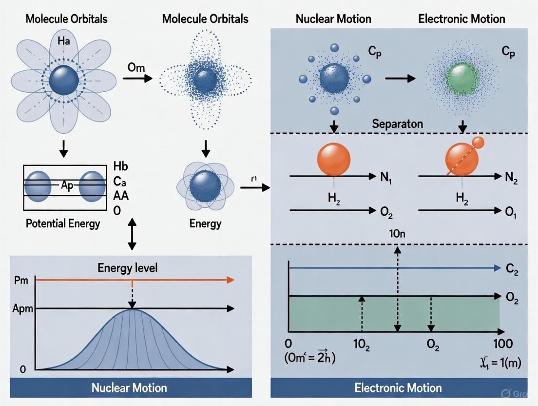
The following diagram illustrates the conceptual separation and energy flow in the Born-Oppenheimer approximation:
Diagram 1: Born-Oppenheimer approximation workflow showing the separation of electronic and nuclear motions.
When the Approximation Breaks Down: Limitations and Breakdown Conditions
Conditions for BO Validity and Vibronic Coupling
The Born-Oppenheimer approximation remains valid when electronic potential energy surfaces are well-separated, satisfying the condition:
[ E0(\mathbf{R}) \ll E1(\mathbf{R}) \ll E_2(\mathbf{R}) \ll \cdots \quad \text{for all } \mathbf{R} ]
Under these conditions, nuclear motion occurs predominantly on a single electronic surface without significant transitions between surfaces [2]. However, this approximation fails when electronic states become degenerate or nearly degenerate, leading to what is known as "vibronic coupling" [6].
Breakdown occurs specifically when:
- Surface crossings or avoided crossings: Electronic states become close in energy, typically at specific nuclear configurations
- Conical intersections: Points where electronic states are exactly degenerate, creating a funnel for rapid non-adiabatic transitions
- Significant non-adiabatic coupling: When the nuclear kinetic energy operator creates substantial mixing between electronic states
The mathematical manifestation of breakdown appears in the form of non-adiabatic coupling terms:
[ \Lambda{kl} = \langle \chik | Tn | \chil \rangle + \sum{A} \frac{1}{MA} \langle \chik | \nablaA \chil \rangle \cdot \nablaA ]
These terms are typically neglected in the BO approximation but become significant when electronic states are close in energy [2]. In such cases, the complete wavefunction must be expressed as a sum of products:
[ \Psi(\mathbf{r}, \mathbf{R}) = \sum{k=1}^K \chik(\mathbf{r}; \mathbf{R}) \phi_k(\mathbf{R}) ]
where the summation includes multiple electronic states, and the nuclear wavefunctions (\phi_k(\mathbf{R})) are coupled through the non-adiabatic operators [2].
Table 2: Conditions for Born-Oppenheimer Approximation Validity and Breakdown
| Scenario | Electronic Structure | Nuclear Dynamics | BO Approximation | Examples |
|---|---|---|---|---|
| Well-separated ground state | (E0 \ll E1) | Adiabatic on ground PES | Valid | Stable organic molecules at room temperature |
| Low-energy excited states | (E1 ) slightly > (E0) | Possible weak coupling | Mostly valid | Fluorescent dyes, some photochemical processes |
| Near-degenerate states | (E1 \approx E0) at some R | Strong non-adiabatic coupling | Breaks down | Conical intersections in photoisomerization |
| Exact degeneracy | (E1 = E0) at point R | Ultrafast transitions | Completely fails | Conical intersections, Jahn-Teller systems |
Experimental and Computational Detection of Breakdown
The breakdown of the BO approximation manifests in several experimental and computational contexts:
- Spectroscopic signatures: Unexpected band shapes, anomalous vibrational progressions, or forbidden transitions appearing in electronic spectra
- Reactivity anomalies: Reaction products or rates that deviate significantly from single-surface predictions
- Ultrafast dynamics: Femtosecond to picosecond timescale processes indicating rapid transitions between electronic states
Computationally, breakdown is detected through:
- Significant magnitude of non-adiabatic coupling vectors
- Small energy gaps between electronic states during dynamics simulations
- Failure of single-reference electronic structure methods
The following diagram illustrates the key differences between the Born-Oppenheimer regime and its breakdown:
Diagram 2: Conditions leading to Born-Oppenheimer approximation validity versus breakdown.
Methodologies and Experimental Protocols
Computational Verification Protocols
Electronic Structure Calculations for Potential Energy Surfaces
Computational verification of the BO approximation's validity involves detailed mapping of potential energy surfaces and their couplings:
Multi-reference electronic structure methods: Utilize complete active space self-consistent field (CASSCF) or multi-reference configuration interaction (MRCI) calculations to properly describe near-degenerate electronic states [6]
Non-adiabatic coupling elements: Compute the derivative coupling vectors ( \langle \chik | \nablaR \chi_l \rangle ) between electronic states using response theory or finite difference methods
Dynamics simulations: Implement either:
Conical intersection optimization: Locate and characterize points of exact degeneracy between electronic states using gradient-based search algorithms
Protocol for Assessing BO Approximation Validity:
- Perform geometry optimization on ground and excited states
- Calculate energy gaps between electronic states along relevant nuclear coordinates
- Compute non-adiabatic coupling strengths at geometries where energy gaps are small
- Estimate coupling magnitudes relative to nuclear kinetic energy
- For small gaps and strong couplings, employ beyond-BO dynamics methods
Spectroscopic Detection Methods
Experimental verification of BO breakdown employs advanced spectroscopic techniques:
Time-Resolved Photoelectron Spectroscopy (TRPES)
- Pump-probe methodology with femtosecond time resolution
- Maps electronic population transfer following photoexcitation
- Directly observes non-adiabatic transitions through changing electron kinetic energy distributions
Two-Dimensional Electronic Spectroscopy (2DES)
- Reveals couplings between electronic states through cross-peaks
- Tracks energy flow between states on ultrafast timescales
- Provides both frequency and time resolution for complete dynamical picture
Vibronic Spectroscopy in Jet-Cooled Molecules
- High-resolution spectroscopy of cold molecules eliminates thermal broadening
- Direct observation of vibrational-electronic (vibronic) coupling patterns
- Quantifies Herzberg-Teller coupling contributions through intensity borrowing
Table 3: Essential Computational Tools for Born-Oppenheimer and Beyond-BO Simulations
| Tool Category | Specific Software/Methods | Primary Function | Application Context |
|---|---|---|---|
| Electronic Structure Packages | Gaussian, GAMESS, ORCA, Q-Chem | PES calculation, geometry optimization | BO validity assessment, ground state dynamics |
| Multi-reference Methods | MOLPRO, MOLCAS, COLUMBUS | Diabatic representation, conical intersection search | Near-degeneracy regions, photochemical reactions |
| Non-adiabatic Dynamics | SHARC, Newton-X, Tully's FSSH | Trajectory surface hopping simulations | BO breakdown regimes, ultrafast photodynamics |
| Wavepacket Propagation | MCTDH, Wavepacket | Quantum nuclear dynamics | Vibronic spectroscopy, light-induced processes |
| Vibronic Coupling Models | VCHAM, Vibronic | Model Hamiltonian parameterization | Systematic studies of BO breakdown patterns |
Applications in Pharmaceutical Research and Drug Development
Mass Spectrometry and Molecular Imaging
The principles underlying the Born-Oppenheimer approximation find practical application in pharmaceutical research through advanced analytical techniques. Mass spectrometry imaging (MSI) has emerged as a powerful tool for untargeted investigation of spatial distribution of molecular species in biological samples [12]. This technique enables imaging of thousands of molecules—including metabolites, lipids, peptides, proteins, and glycans—in a single experiment without labeling [12].
In MSI experiments, the mass spectrometer ionizes molecules on a sample surface and collects a mass spectrum at each pixel, with spatial resolution defined by pixel size [12]. The resulting data allows researchers to extract intensity information for specific mass-to-charge (m/z) values and create heat map images depicting molecular distributions throughout the sample [12]. This application implicitly relies on the BO framework through its dependence on molecular ionization potentials and fragmentation patterns that are interpreted through computational chemistry methods grounded in the BO approximation.
High-Throughput Screening in Drug Discovery
Recent technological developments have revolutionized the application of mass spectrometry for high-throughput (HT) screening in early drug discovery pipelines [9]. HT-MS platforms enable label-free detection of biomolecules in screening assays, expanding the breadth of targets for which HT assays can be developed compared to traditional approaches [9].
These MS-based screening methods include:
- Affinity selection mass spectrometry: Identifies target binders from complex mixtures
- Biochemical activity screening: Directly measures enzyme substrates and products
- Cellular phenotypic screening: Detects compound-induced changes in cellular metabolism
The BO approximation facilitates the computational drug design component of these efforts by enabling efficient prediction of drug-target interactions, binding affinities, and metabolic stability through quantum mechanical calculations that would be prohibitively expensive without the separation of electronic and nuclear degrees of freedom.
The Born-Oppenheimer approximation remains one of the most successful and widely applied concepts in molecular quantum mechanics, with its core physical insight—leveraging the mass disparity between nuclei and electrons—continuing to enable advances across chemical physics, materials science, and pharmaceutical research. While modern computational methods have developed sophisticated approaches to handle cases where the approximation breaks down, the BO framework provides the essential foundation upon which our understanding of molecular structure and dynamics is built.
In pharmaceutical contexts, the BO approximation enables everything from molecular property prediction to drug-receptor interaction modeling, while its limitations in describing non-adiabatic processes inform research in photodynamic therapy and radiation-induced damage. As computational power increases and experimental techniques achieve greater temporal and spatial resolution, the fundamental insight of separated electronic and nuclear motions continues to guide both theoretical development and practical applications in molecular systems research.
In quantum chemistry, the description of molecular systems begins with the molecular Hamiltonian, which encapsulates the total energy of all electrons and nuclei. For a molecule with multiple electrons and nuclei, the complete, non-relativistic Coulomb Hamiltonian is expressed as follows [13]: [ \hat{H}{\text{total}} = \hat{T}n + \hat{T}e + \hat{U}{en} + \hat{U}{ee} + \hat{U}{nn} ] where the terms respectively represent the nuclear kinetic energy, the electronic kinetic energy, the electron-nucleus attraction, the electron-electron repulsion, and the nucleus-nucleus repulsion [13]. The challenge in solving the corresponding Schrödinger equation arises from the coupled nature of the nuclear and electronic coordinates. The Born-Oppenheimer (BO) approximation provides the foundational framework for decoupling these motions, thereby simplifying the problem into more tractable parts. This separation is justified by the significant disparity in mass between nuclei and electrons, which causes nuclei to move on a much slower timescale, allowing electrons to be treated as moving within a field of effectively stationary nuclei [2] [14] [15]. This whitepaper details the mathematical formalism of separating the Hamiltonian and derives the central equation for electronic structure theory: the electronic Schrödinger equation.
Mathematical Decomposition of the Molecular Hamiltonian
The Full Coulomb Hamiltonian
The Coulomb Hamiltonian is written explicitly in atomic units as [2] [13]: [ \hat{H}{\text{total}} = -\sum{A} \frac{1}{2MA}\nabla{A}^{2} - \sum{i} \frac{1}{2}\nabla{i}^{2} - \sum{i,A} \frac{ZA}{r{iA}} + \sum{i>j} \frac{1}{r{ij}} + \sum{B>A} \frac{ZA ZB}{R{AB}} ] Here, the indices ( A, B ) refer to nuclei, and ( i, j ) refer to electrons. The terms ( MA ) and ( ZA ) are the mass and atomic number of nucleus ( A ), while ( r{iA} ), ( r{ij} ), and ( R{AB} ) denote electron-nucleus, electron-electron, and nucleus-nucleus distances, respectively [2]. The Laplacian operators ( \nabla{A}^{2} ) and ( \nabla{i}^{2} ) represent the kinetic energy of nuclei and electrons.
Table 1: Components of the Full Molecular Coulomb Hamiltonian
| Term Symbol | Mathematical Expression | Physical Description |
|---|---|---|
| ( \hat{T}_n ) | ( -\sum{A} \frac{1}{2MA}\nabla_{A}^{2} ) | Kinetic energy of the nuclei |
| ( \hat{T}_e ) | ( -\sum{i} \frac{1}{2}\nabla{i}^{2} ) | Kinetic energy of the electrons |
| ( \hat{U}_{en} ) | ( -\sum{i,A} \frac{ZA}{r_{iA}} ) | Attractive potential between electrons and nuclei |
| ( \hat{U}_{ee} ) | ( \sum{i>j} \frac{1}{r{ij}} ) | Repulsive potential between electrons |
| ( \hat{U}_{nn} ) | ( \sum{B>A} \frac{ZA ZB}{R{AB}} ) | Repulsive potential between nuclei |
The Born-Oppenheimer Approximation and Hamiltonian Separation
The Born-Oppenheimer approximation states that the total wavefunction can be separated into a product of a nuclear wavefunction and an electronic wavefunction [2]: [ \Psi{\text{total}}(\mathbf{r}, \mathbf{R}) = \psi{\text{nuclear}}(\mathbf{R}) \cdot \psi{\text{electronic}}(\mathbf{r}; \mathbf{R}) ] A critical step is recognizing that the nuclear kinetic energy term ( \hat{T}n ) is negligible when solving for the electronic wavefunction. This is because the mass of a nucleus is thousands of times greater than that of an electron, leading to much smaller accelerations for a given force [14] [15]. Consequently, the nuclei can be treated as fixed, classical point charges when determining the electronic state. This leads to the so-called clamped-nuclei Hamiltonian or electronic Hamiltonian ( \hat{H}e ) [2] [13], obtained by omitting ( \hat{T}n ) from the full Hamiltonian: [ \hat{H}e(\mathbf{r}, \mathbf{R}) = \hat{T}e + \hat{U}{en} + \hat{U}{ee} + \hat{U}{nn} ] It is crucial to note that the electronic Hamiltonian ( \hat{H}e ) depends parametrically on the nuclear coordinates ( \mathbf{R} ). This means ( \mathbf{R} ) is not a quantum mechanical variable in the electronic equation but a set of fixed parameters. The nuclear repulsion term ( \hat{U}_{nn} ) is a constant for a fixed nuclear configuration [2].
Diagram 1: Workflow for separating the Hamiltonian via the Born-Oppenheimer approximation, showing the derivation of the electronic Schrödinger equation and the potential energy surface.
The Electronic Schrödinger Equation
Definition and Eigenvalue Problem
With the electronic Hamiltonian defined, the electronic Schrödinger equation is formulated as follows [2] [15]: [ \hat{H}e(\mathbf{r}, \mathbf{R}) \chik(\mathbf{r}; \mathbf{R}) = E{e,k}(\mathbf{R}) \chik(\mathbf{r}; \mathbf{R}) ] Here, ( \chik(\mathbf{r}; \mathbf{R}) ) is the electronic wavefunction for the ( k )-th electronic state, and ( E{e,k}(\mathbf{R}) ) is the corresponding electronic energy eigenvalue. Both quantities depend parametrically on the nuclear coordinates ( \mathbf{R} ). The electronic energy includes contributions from electron kinetics, all Coulomb interactions, and crucially, the constant nuclear repulsion term ( U{nn} ). The total energy for a given electronic state at a fixed nuclear configuration is ( E{e,k}(\mathbf{R}) ) [2].
The Potential Energy Surface (PES)
By solving the electronic Schrödinger equation for a range of nuclear configurations, one maps out a Potential Energy Surface (PES), ( E_{e,k}(\mathbf{R}) ). This surface governs the motion of the nuclei [2] [14]. The PES is a central concept in quantum chemistry, as it allows for the subsequent treatment of nuclear motion (vibrations, rotations) and the analysis of molecular geometry, stability, and reaction pathways [14].
Computational Methodologies and Protocols
Standard Workflow for Electronic Structure Calculation
The theoretical separation described above translates into a standard computational workflow in quantum chemistry.
- Define Molecular Geometry: Specify the atomic symbols ( {Z_A} ) and nuclear coordinates ( \mathbf{R} ) for the system [16].
- Select Atomic Basis Set: Choose a set of basis functions (e.g., Gaussian-type orbitals) to represent the molecular orbitals [16].
- Solve the Electronic Problem: For the fixed nuclear configuration, compute the electronic wavefunction ( \chik ) and energy ( E{e,k} ). This is typically done at the Hartree-Fock (HF) level or with post-HF methods to account for electron correlation [16].
- Construct the PES: Repeat the electronic structure calculation over a grid of nuclear coordinates to build the PES [2].
- Solve Nuclear Dynamics: Use the PES ( E_{e,k}(\mathbf{R}) ) in a nuclear Schrödinger equation to study vibrations and rotations, or in classical molecular dynamics simulations [14].
Advanced Implementation: Second Quantization and Quantum Computing
For advanced simulations, particularly on quantum computers, the electronic Hamiltonian is often transformed into the second quantization formalism [16]: [ \hat{H}e = \sum{pq} h{pq} cp^\dagger cq + \frac{1}{2} \sum{pqrs} h{pqrs} cp^\dagger cq^\dagger cr cs ] Here, ( cp^\dagger ) and ( cq ) are fermionic creation and annihilation operators, and ( h{pq} ) and ( h_{pqrs} ) are one- and two-electron integrals computed in a molecular orbital basis. This fermionic Hamiltonian can then be mapped to a qubit Hamiltonian using transformations like the Jordan-Wigner or Bravyi-Kitaev encoding, enabling quantum algorithm deployment [16].
Table 2: Key Research Reagent Solutions for Electronic Structure Calculations
| Reagent / Computational Tool | Function in the Research Process |
|---|---|
| Atomic Orbital Basis Sets | Serve as basis functions for expanding molecular orbitals, critical for representing the electronic wavefunction. |
| Hartree-Fock Solver | Computes the mean-field approximation of the electronic wavefunction and optimizes molecular orbital coefficients. |
| Electronic Integral Packages | Calculate the one- and two-electron integrals ( (h{pq}, h{pqrs}) ) over the chosen basis set, which are the building blocks of the Hamiltonian. |
| Fermion-to-Qubit Mappers (e.g., Jordan-Wigner) | Transform the second-quantized electronic Hamiltonian into a Pauli spin operator form executable on a quantum processor. |
| Classical Quantum Chemistry Packages (e.g., PySCF, Q-Chem) | Perform the complete workflow from molecular structure to PES construction using high-performance computing resources. |
Diagram 2: Detailed protocol for building the electronic Hamiltonian in a form suitable for quantum simulations, from molecular structure to a solvable qubit Hamiltonian.
Limitations and Beyond the Born-Oppenheimer Formalism
The BO approximation is highly successful but fails when electronic states become nearly degenerate, such as at conical intersections. In these regions, the coupling terms involving nuclear momentum operators ( \hat{P}{A\alpha} = -i \frac{\partial}{\partial R{A\alpha}} ) acting on the electronic wavefunction can no longer be ignored [2] [17]. This breakdown necessitates beyond-BO methods. One advanced approach is the exact factorization framework, which expresses the total wavefunction as a single product ( \Psi(\mathbf{r}, \mathbf{R}, t) = \chi(\mathbf{R}, t) \Phi_{\mathbf{R}}(\mathbf{r}, t) ) without approximation [17]. This leads to coupled equations for the nuclear and conditional electronic wavefunctions, introducing time-dependent vector and scalar potentials that mediate the exact electron-nuclear coupling, providing a formally exact path for simulating coupled dynamics [17].
The mathematical formalism of separating the full molecular Hamiltonian via the Born-Oppenheimer approximation is a cornerstone of modern molecular quantum mechanics. It reduces the intractable coupled problem into a sequence of manageable steps: defining an electronic Hamiltonian that depends parametrically on nuclear coordinates, solving the electronic Schrödinger equation to generate a potential energy surface, and finally treating nuclear motion on this surface. This formalism enables the computational prediction of molecular structure, properties, and reactivity, forming the theoretical foundation for a vast range of applications in drug discovery, materials science, and chemical physics. While the BO approximation is remarkably effective, ongoing research into non-adiabatic processes and beyond-BO methods like the exact factorization framework continues to expand the frontiers of simulating coupled electron-nuclear dynamics.
The Born-Oppenheimer (BO) approximation, introduced in 1927 by Max Born and J. Robert Oppenheimer, represents one of the most foundational concepts in quantum chemistry and molecular physics [2] [18]. This approximation exploits the significant mass disparity between atomic nuclei and electrons to separate their motions, thereby transforming the intractable many-body molecular Schrödinger equation into a solvable problem [19]. This whitepaper traces the historical development of the BO approximation from its theoretical origins to its modern status as an indispensable tool in computational chemistry, with a specific focus on its applications and limitations in molecular systems research and drug discovery. We provide a detailed analysis of its theoretical underpinnings, quantitative performance across computational methods, and protocols for its application in contemporary research, framing this discussion within a broader thesis on its enduring impact on molecular sciences.
The year 1927 was a period of intense development in quantum mechanics, just one year after Erwin Schrödinger published his famous wave equation [20]. In this fertile environment, the 23-year-old J. Robert Oppenheimer, working under the guidance of Max Born, proposed the approximation that would bear their names [2] [18]. Although the theory is jointly attributed, most historians recognize that the majority of the work was carried out by Oppenheimer himself [18].
The fundamental challenge addressed by the BO approximation was the quantum mechanical description of molecules, which requires defining the positions and movements of all atomic nuclei and electrons and computing the complex charge interactions between these particles [18]. Solving the molecular Schrödinger equation presented a formidable challenge—it could not be solved exactly even for the simplest molecule, H₂⁺, consisting of just two protons and one electron [18].
Oppenheimer's key insight was recognizing that atomic nuclei are much heavier than electrons, with a single proton weighing nearly 2,000 times more than an electron [18]. This mass disparity, on the order of ~10³, meant that nuclei move significantly slower than electrons [20] [21]. Consequently, electrons effectively instantaneously adjust to nuclear motion, allowing scientists to treat nuclei as nearly stationary while solving the Schrödinger equation exclusively for electrons [2] [19]. This conceptual separation dramatically simplified the complexity of quantum mechanical calculations for molecules.
Theoretical Framework and Computational Workflow
Mathematical Formulation
The BO approximation begins with the complete molecular Hamiltonian, which includes all kinetic and potential energy terms for nuclei and electrons [2] [21]. The approximation recognizes the large difference between electron mass and the masses of atomic nuclei, and correspondingly the time scales of their motion [2].
The total wave function is expressed as a product of electronic and nuclear wave functions [2] [21]:
Ψ_total(r,R) = ψ_electronic(r; R) ψ_nuclear(R)
Here, r represents all electronic coordinates and R represents all nuclear coordinates [21]. The electronic wave function ψ_electronic depends parametrically on the nuclear positions R [2] [21]. This parametric dependence is continuous and differentiable, though the derivatives are generally non-zero and lead to coupling terms [2].
The molecular Schrödinger equation is separated into two coupled equations [2] [21]:
The Electronic Schrödinger Equation: For fixed nuclear positions, one solves:
H_e χ_k(r; R) = E_k(R) χ_k(r; R)whereH_eis the electronic Hamiltonian,χ_kis the electronic wavefunction for state k, andE_k(R)is the electronic energy as a function of nuclear configuration [2].The Nuclear Schrödinger Equation: Using the electronic energy as a potential, one solves:
[T_n + E_e(R)] ϕ(R) = E ϕ(R)whereT_nis the nuclear kinetic energy operator [2].
Computational Workflow and Visualization
The following diagram illustrates the standard computational workflow enabled by the Born-Oppenheimer approximation:
This computational workflow demonstrates how the BO approximation enables practical quantum chemistry calculations. The electronic structure calculation forms the foundation, repeated for various nuclear arrangements to map out a Potential Energy Surface (PES) [19]. This surface then dictates how the nuclei move, vibrate, and rotate [19]. Minima on this surface correspond to stable molecular structures (equilibrium geometries), saddle points represent transition states for chemical reactions, and the overall topography governs molecular vibrations and reaction pathways [19].
The Scientist's Toolkit: Essential Computational Methods
Table 1: Quantum Chemical Methods Relying on the BO Approximation
| Method | Theoretical Basis | Key Features | Computational Scaling | Typical Applications |
|---|---|---|---|---|
| Hartree-Fock (HF) | Wavefunction theory using single Slater determinant [22] [23] | Neglects electron correlation; self-consistent field (SCF) approach [22] | O(N⁴) with basis set size [23] | Baseline electronic structures; starting point for correlated methods [23] |
| Density Functional Theory (DFT) | Uses electron density rather than wavefunction [22] [23] | Includes approximate exchange-correlation functional; good accuracy/efficiency balance [22] | O(N³) to O(N⁴) [22] | Most widely used QM method; molecular structures, properties, reaction pathways [23] |
| Møller-Plesset Perturbation Theory (MP2) | Post-HF electron correlation treatment [22] | Accounts for electron correlation via perturbation theory [22] | O(N⁵) [22] | More accurate binding energies; dispersion interactions [22] |
| Coupled Cluster (e.g., CCSD(T)) | Post-HF using exponential cluster operator [22] | "Gold standard" for molecular energy calculations [22] | O(N⁷) or higher [22] | High-accuracy reference calculations; benchmark studies [22] |
The computational methods summarized in Table 1 all fundamentally rely on the BO approximation, demonstrating its pervasive influence across quantum chemistry. The choice of method involves a trade-off between accuracy and computational cost, with more accurate methods typically requiring significantly more resources [22].
Quantitative Performance and Methodological Comparisons
Computational Efficiency Gains
The BO approximation provides dramatic reductions in computational complexity. For illustration, consider the benzene molecule (C₆H₆), which consists of 12 nuclei and 42 electrons [2]. The full Schrödinger equation requires solving for 3 × 12 = 36 nuclear plus 3 × 42 = 126 electronic coordinates, totaling 162 variables [2]. Since computational complexity increases faster than the square of the number of coordinates, the full problem would require solving at least 162² = 26,244 variables [2].
Using the BO approximation, this problem is separated into [2]:
- Electronic problem: 126 electronic coordinates, solved multiple times for different nuclear configurations
- Nuclear problem: 36 nuclear coordinates, solved once on the pre-computed potential energy surface
This separation reduces the computational complexity from a single O(162²) problem to multiple O(126²) problems plus one O(36²) problem, representing a substantial reduction in computational demand [2].
Accuracy Comparison Across Methods
Table 2: Performance Benchmarks of Quantum Chemistry Methods
| Method | Bond Length Accuracy | Binding Energy Error | Computational Time (Relative) | Key Limitations |
|---|---|---|---|---|
| Molecular Mechanics (MM) | Poor for unusual bonding features [22] | Very poor at conformational prediction [22] | Fraction of a second [22] | Cannot model polarizability, charge transfer, or bond breaking/formation [22] |
| Semiempirical Methods | Moderate [22] | Moderate [22] | Seconds to minutes [22] | Parameter-dependent; limited transferability [22] |
| Hartree-Fock (HF) | Bonds typically too long and weak [22] | Underestimates by 20-30% for non-covalent interactions [22] | Minutes to hours [22] | Neglects electron correlation; poor for dispersion forces [23] |
| Density Functional Theory (DFT) | Good with appropriate functional [22] [23] | ~1-3 kcal/mol error with modern functionals [23] | Hours to days [22] | Exchange-correlation functional choice critical; delocalization errors [23] |
| MP2 and Coupled Cluster | Excellent [22] | <1 kcal/mol for CCSD(T) [22] | Days to weeks [22] | Computationally prohibitive for large systems [22] |
The data in Table 2 illustrates the Pareto frontier of quantum chemistry methods, where increasing accuracy comes at the cost of greater computational resources [22]. Molecular mechanics methods (force fields) are fast but lack quantum mechanical accuracy, while high-level wavefunction methods provide exceptional accuracy but at extreme computational cost [22].
Applications in Drug Discovery and Molecular Design
Key Application Areas
The BO approximation enables numerous critical applications in drug discovery and molecular design:
- Equilibrium Geometry Prediction: Finding the lowest energy structure on the potential energy surface, which corresponds to stable molecular conformations [19].
- Vibrational Frequency Analysis: Analyzing the curvature of the PES around a minimum to predict molecular vibrational spectra, which aids in structure validation and characterization [19].
- Reaction Pathway Studies: Identifying transition states and activation barriers on the PES to understand and predict chemical reactivity and reaction mechanisms [19].
- Binding Affinity Calculations: Modeling protein-ligand interactions and computing binding energies to optimize drug candidate potency [23].
Experimental Protocol: DFT Calculation for Drug Design
For researchers applying these methods, here is a detailed protocol for a typical DFT calculation in drug discovery:
System Preparation
- Obtain initial molecular coordinates from crystallography, molecular docking, or molecular mechanics optimization
- Define the molecular system including protonation states relevant to physiological conditions
- For large systems, consider QM/MM approaches where the active site is treated with QM and the protein environment with molecular mechanics [23]
Method Selection
Calculation Execution
- Perform geometry optimization to locate minima on the PES
- Confirm stationary points with frequency calculations (no imaginary frequencies for minima, one for transition states)
- Compute single-point energies with higher-level methods if needed
Analysis
- Analyze molecular orbitals, electrostatic potentials, and electron densities
- Calculate binding energies using appropriate counterpoise corrections for basis set superposition error
- Compare with experimental data (spectra, binding affinities, reaction rates) for validation
This protocol enables researchers to predict molecular properties, binding modes, and reactivities that inform drug design decisions [23].
Limitations and Breakdown of the Approximation
When the BO Approximation Fails
Despite its widespread success, the BO approximation has well-established limitations. It may break down in specific scenarios, such as light-driven chemical reactions or processes enabling vision in animals [18]. The breakdown occurs when the central assumption of separable electronic and nuclear motion becomes invalid [21].
The most dramatic failures occur at conical intersections, points in nuclear configuration space where two or more electronic potential energy surfaces touch or become degenerate [19] [21]. Near these points, non-adiabatic coupling terms become large, and the assumption of separate electronic and nuclear motion is entirely invalid [19]. Dynamics passing through conical intersections are ultrafast and play a crucial role in determining reaction outcomes, photostability, and energy relaxation pathways [19].
The formal breakdown can be understood mathematically through the nuclear derivative couplings that are neglected in the standard BO approximation [21]. The complete molecular wavefunction including multiple electronic states is:
Ψ(r,R) = Σ ψ_j(r; R) χ_j(R)
Substituting this into the full Schrödinger equation reveals coupling terms of the form [21]:
⟨ψ_i|T_N|ψ_j⟩- kinetic coupling between electronic statesΣ_α -ℏ²/2m_α ⟨ψ_i|∇_R_α|ψ_j⟩·∇_R_α- non-adiabatic coupling operators
These terms are responsible for transitions between electronic states and become significant when electronic energy levels become close or degenerate [21].
Advanced Methods Beyond BO
Table 3: Methods for Handling BO Breakdown
| Method | Approach | Applications | Computational Cost |
|---|---|---|---|
| Trajectory Surface Hopping | Classical nuclei with stochastic hops between PESs [19] | Photochemical reactions, electron transfer [19] | Moderate to high |
| Multi-Configuration Time-Dependent Hartree (MCTDH) | Quantum dynamics for nuclei on multiple PESs [19] | Accurate quantum dynamics in small systems [19] | Very high |
| Nuclear-Electronic Orbital (NEO) Theory | Treats specified nuclei (e.g., protons) quantum mechanically alongside electrons [24] | Proton transfer, hydrogen bonding [24] | High |
| Multi-Component Unitary Coupled Cluster (mcUCC) | Quantum computing approach treating electrons and nuclei simultaneously [24] | Small model systems; proof of concept [24] | Extremely high |
For systems where the BO approximation fails, the methods in Table 3 provide more accurate treatments. Recent advances include multicomponent quantum simulations that treat both electronic and nuclear quantum effects simultaneously, implemented on quantum hardware with error mitigation techniques [24].
The following diagram illustrates the conceptual relationship between different computational approaches for molecular systems:
Emerging Directions
The future of the BO approximation in molecular research involves both pushing its boundaries and developing methods for its limitations:
Quantum Computing: Quantum computers hold promise for enhancing computational quantum chemistry by enabling faster calculations on increasingly complex molecular systems [18] [24]. Recent demonstrations of error-mitigated multicomponent simulations on quantum hardware represent early steps toward this future [24].
Machine Learning Force Fields: Machine learning approaches are being developed to learn potential energy surfaces from quantum mechanical data, maintaining accuracy while dramatically reducing computational cost [22].
Non-Adiabatic Dynamics: Methods for simulating dynamics beyond the BO approximation continue to advance, enabling more accurate modeling of photochemical processes, charge transfer, and other electronically non-adiabatic phenomena [19].
From its inception in 1927 to the present day, the Born-Oppenheimer approximation has evolved from a theoretical concept to a cornerstone of modern computational chemistry and molecular design. Its simplicity—separating electronic and nuclear motion based on mass disparity—belies its transformative impact, enabling the practical application of quantum mechanics to molecular systems of biological and technological relevance.
While the approximation has limitations, particularly in photochemistry and processes involving multiple electronic states, it remains the foundation upon which most quantum chemical methods are built. Its enduring legacy is reflected in its pervasive use across chemistry, materials science, and drug discovery, where it continues to enable researchers to understand and predict molecular structure, properties, and reactivity. As computational power grows and new theoretical approaches emerge, the BO approximation will continue to serve as both a practical tool and a conceptual framework for understanding the quantum nature of molecules.
From Theory to Therapy: Applying Born-Oppenheimer Methods in Computational Drug Design
Computational chemistry plays a critical role in advancing molecular science by bridging theoretical frameworks and experimental observations, providing detailed insight into the structural, electronic, and reactive properties of molecules and materials [25]. The field relies on a hierarchical approach to modeling, employing methods of varying computational cost and accuracy to address different scientific questions. At the core of this hierarchy lies the Born-Oppenheimer (BO) approximation, which serves as the fundamental tenet enabling most practical computational chemistry applications [6] [26]. This approximation introduces a hierarchy in electron-nuclear interactions by separating the motion of electrons from that of the nuclei, allowing chemists to picture molecules as nuclei connected by electrons rather than as a homogeneous "soup" of interacting particles [6].
Despite its central importance, the BO approximation is often misinterpreted. Widespread claims within the chemistry community incorrectly imply that this approximation enforces nuclei to be frozen or treated as classical particles [6]. In reality, the BO approximation does not require frozen nuclei; rather, it provides a mathematical framework for separating electronic and nuclear motions, forming the basis for potential energy surfaces on which nuclei move [6] [26]. When this approximation breaks down—as in photochemical processes or systems involving proton tunneling—more sophisticated methods beyond BO become necessary [27] [28]. This review examines the computational hierarchy from quantum mechanics to multi-scale QM/MM methods, framed within the foundational context of the Born-Oppenheimer approximation in molecular systems research.
Theoretical Framework: The Born-Oppenheimer Approximation
The Born-Oppenheimer approximation finds its roots in solving the molecular Schrödinger equation, which describes the quantum mechanical behavior of a molecule comprising multiple electrons and nuclei [6]. The full molecular Hamiltonian operator, as defined in atomic units, includes kinetic energy terms for all nuclei and electrons, as well as potential energy terms for all interparticle interactions [26]. Solving this equation directly is mathematically intractable for all but the simplest systems due to the coupled nature of all particles.
The BO approximation addresses this challenge by exploiting the significant mass disparity between electrons and nuclei. Since nuclei are thousands of times heavier than electrons, their motion is considerably slower [26]. This separation of time scales allows for the approximation that electrons instantaneously adjust their distribution to any new configuration of the nuclei. Mathematically, this enables the separation of the total molecular wavefunction into electronic and nuclear components [26]. The electronic Schrödinger equation is solved for fixed nuclear positions, generating a potential energy surface on which the nuclei subsequently move [6] [23].
This theoretical framework enables the concept of molecular geometry, bonding, and potential energy surfaces that underpin modern computational chemistry. However, in systems where electronic and nuclear motions become strongly coupled—such as in conical intersections, proton-coupled electron transfer, or systems with significant hydrogen tunneling—the BO approximation breaks down, necessitating more sophisticated treatments that explicitly account for non-adiabatic effects [27] [28]. For most chemical applications, including drug discovery and materials design, the BO approximation remains the essential starting point that makes computational modeling feasible [23].
Quantum Mechanical Methods
Fundamental Principles and Methodological Spectrum
Quantum mechanical (QM) methods serve as the theoretical bedrock of computational chemistry, providing a rigorous framework for understanding molecular structure, reactivity, and properties at the atomic level [25]. These methods solve the electronic Schrödinger equation under the Born-Oppenheimer approximation, calculating the electronic structure of molecules for fixed nuclear positions. The fundamental goal is to determine molecular wavefunctions and energies, from which all other molecular properties can be derived.
The methodological spectrum of quantum chemistry encompasses various approaches with distinct trade-offs between computational efficiency and accuracy. Ab initio (first-principles) methods derive molecular properties directly from physical principles without empirical parameters [25]. These include:
- Hartree-Fock (HF) method: One of the earliest quantum chemical models that approximates electrons as independent particles moving in an averaged electrostatic field [25]. While widely used as a reference for more sophisticated techniques, its neglect of electron correlation limits predictive accuracy for interaction energies and bond dissociation [25] [23].
- Post-Hartree-Fock methods: Include Møller-Plesset perturbation theory (MP2), Configuration Interaction (CI), and Coupled Cluster (CC) theory, which address electron correlation directly and offer greater accuracy [25]. The Coupled Cluster with Single, Double, and perturbative Triple excitations (CCSD(T)) method is widely regarded as the benchmark for precision in quantum chemistry [25].
- Density Functional Theory (DFT): Shifts the focus from wavefunctions to electron density, reducing computational demands while incorporating electron correlation through exchange-correlation functionals [25] [23]. This balance of cost and accuracy has led to DFT's widespread use for calculating ground-state properties of medium to large molecular systems [25].
Semiempirical quantum chemical methods occupy a middle ground, incorporating approximate integrals and parameterized elements to achieve significantly reduced computational cost, making them valuable for large-scale screening and geometry optimization [25].
Key Developments and Applications
Recent advances in quantum chemistry have enhanced the accuracy and applicability of these methods across chemical research. Improvements to DFT have addressed many of its shortcomings through the development of range-separated and double-hybrid functionals, along with empirical dispersion corrections such as DFT-D3 and DFT-D4 [25]. These refinements have extended DFT's applicability to non-covalent systems, transition states, and electronically excited configurations relevant to catalysis, photochemistry, and materials design [25].
The integration of machine learning with quantum methods has gained significant traction, enabling hybrid models that leverage physics-based approximations and data-driven corrections [25]. Recent developments such as GFN2-xTB offer broad applicability with significantly reduced computational cost [25]. Fragment-based and multi-scale quantum mechanical techniques like the Fragment Molecular Orbital (FMO) approach and ONIOM provide practical strategies for handling large systems by enabling localized quantum treatments of subsystems within broader classical environments [25].
Quantum mechanical methods excel in determining electronic structure of complex molecules, studying photochemistry and excited states, and mapping chemical reaction mechanisms [25]. Techniques including time-dependent DFT (TD-DFT), complete active space self-consistent field (CASSCF), and equation-of-motion coupled-cluster (EOM-CC) approaches offer detailed understanding of light-induced phenomena, electronic excitations, and relaxation processes [25]. These capabilities are central to materials development for applications in photovoltaics, photodynamic therapy, and molecular electronics.
Table 1: Comparison of Major Quantum Mechanical Methods
| Method | Theoretical Foundation | Computational Scaling | Key Strengths | Key Limitations |
|---|---|---|---|---|
| Hartree-Fock (HF) | Wavefunction theory, single Slater determinant | O(N⁴) | Fundamental reference method, physically meaningful orbitals | Neglects electron correlation, poor for dispersion |
| Density Functional Theory (DFT) | Electron density, Hohenberg-Kohn theorems | O(N³) | Favourable cost/accuracy balance, good for geometries and frequencies | Functional dependence, challenges with dispersion and strong correlation |
| MP2 | Wavefunction theory, perturbation theory | O(N⁵) | Accounts for electron correlation, good for non-covalent interactions | Can overbind, sensitive to basis set |
| CCSD(T) | Wavefunction theory, coupled cluster | O(N⁷) | "Gold standard" for chemical accuracy | Prohibitive cost for large systems |
| Semiempirical Methods | Empirical parameterization, simplified integrals | O(N²-N³) | Very fast, applicable to very large systems | Parameter-dependent, transferability issues |
Molecular Mechanics Methods
Force Fields and Parametrization
Molecular mechanics (MM) provides a classical alternative to quantum mechanics by representing molecules as collections of atoms connected by springs, employing empirical potential functions known as force fields to describe the potential energy surface [25]. Unlike QM methods that explicitly treat electrons, MM methods describe molecular systems using a ball-and-spring model based on classical physics, making them computationally efficient for large systems but incapable of modeling bond formation or breaking.
The basic functional form of a typical molecular mechanics force field includes:
- Bond stretching: Described by harmonic potentials that model the energy required to stretch or compress bonds from their equilibrium values
- Angle bending: Represented by harmonic potentials for deviations from equilibrium bond angles
- Torsional potentials: Periodic functions that describe the energy associated with rotation around bonds
- Non-bonded interactions: Include van der Waals interactions (typically modeled by Lennard-Jones potentials) and electrostatic interactions (described by Coulomb's law with partial atomic charges) [25]
Parameterization of force fields involves optimizing these potential functions and their parameters to reproduce experimental data or high-level quantum mechanical calculations [25]. Popular force fields such as AMBER, CHARMM, and OPLS-AA are specifically parameterized for biomolecular simulations and have become standards in the field [23].
Applications and Limitations
Molecular mechanics methods, particularly when coupled with simulation techniques like molecular dynamics (MD) or Monte Carlo, provide efficient large-scale modeling of structural and energetic properties across diverse environments [25]. They enable the simulation of biomolecular systems with hundreds of thousands of atoms over microsecond to millisecond timescales, capturing essential conformational dynamics, ligand binding, and protein folding events that remain inaccessible to quantum methods.
Classical MD simulations provide crucial insights into dynamic processes, offering perspectives that complement experimental observations [29]. However, the accuracy of MM simulations is fundamentally limited by the quality of the force field and its inherent inability to describe electronic phenomena such as charge transfer, polarization effects, and chemical reactions [30]. These limitations restrict MM to applications where the electronic structure remains largely invariant, making them unsuitable for studying chemical reactivity, excitation processes, or systems where explicit electron effects are paramount.
Hybrid QM/MM Methodologies
Theoretical Foundations and Embedding Schemes
Hybrid quantum mechanics/molecular mechanics (QM/MM) methodologies represent a powerful multiscale approach that combines the strengths of both QM and MM methods [29]. These techniques partition the system into a small, chemically active region treated quantum mechanically (where bond formation/breaking or electronic excitations occur) and a larger environment described using molecular mechanics, thereby achieving quantum accuracy for the reactive center while maintaining computational efficiency for the full system [29].
The total energy in a QM/MM calculation is typically expressed as:
[ E{\text{total}} = E{\text{QM}} + E{\text{MM}} + E{\text{QM/MM}} ]
where (E{\text{QM}}) is the energy of the quantum region, (E{\text{MM}}) is the energy of the classical region, and (E_{\text{QM/MM}}) represents the interaction between the two regions [29].
Three primary embedding schemes define how the QM and MM regions interact:
- Mechanical Embedding: The simplest approach where the QM region interacts with fixed MM charges via classical electrostatics, but the MM charges do not polarize the QM wavefunction [31]
- Electrostatic Embedding: The most common approach where the external potential from MM point charges acts on the QM subsystem and polarizes it, though typically without back-polarization of the MM subsystem [29]
- Polarized Embedding: More sophisticated approaches that allow mutual polarization between QM and MM regions, though these require polarizable force fields and are computationally more demanding
The selection of the QM/MM boundary in covalently bonded systems presents a significant challenge, often addressed through the use of link atoms or localized orbitals to saturate valencies [29].
Implementation and Accelerated Sampling
Implementing efficient QM/MM simulations requires addressing the significant computational cost of solving the QM problem at each MD step [29]. Several strategies have been developed to overcome this limitation:
- Enhanced Sampling Approaches: Techniques such as metadynamics, umbrella sampling, and replica-exchange MD accelerate rare-event observation by applying controlled biases to the system [29]
- Multiple Time Step (MTS) MD: Algorithms that propagate the more expensive QM calculations at larger time steps while treating faster MM motions with shorter steps [29]
- Performance-Optimized Frameworks: Simulation frameworks like MiMiC designed for computational performance and flexibility across diverse computing architectures [29]
Recent methodological advances include the development of adaptive QM/MM-NN MD methods that combine neural network predictions with iterative protocols to achieve ab initio QM/MM accuracy with significantly reduced computational cost [30]. These methods perform direct MD simulations on a neural network-predicted potential energy surface that approximates the ab initio QM/MM potential, with adaptive updates to the network when new configurations are encountered during sampling [30].
Adaptive QM/MM-NN MD Workflow: This iterative protocol combines neural network predictions with high-level QM calculations to achieve accurate sampling at reduced cost [30].
Machine Learning-Enhanced Approaches
ML Potentials and Hierarchical Learning
Machine learning has emerged as a transformative element in computational chemistry, enabling the development of data-driven tools that identify molecular features correlated with target properties, thereby accelerating discovery while minimizing trial-and-error experimentation [25] [32]. ML potentials trained on quantum mechanical data can achieve near-quantum accuracy at significantly reduced computational cost, addressing the sampling limitations of direct QM/MM simulations.
A particularly powerful approach involves hierarchical machine learning frameworks that systematically distill knowledge from high-fidelity quantum calculations into increasingly efficient, machine-learned quantum Hamiltonians [32]. This hierarchical structure typically follows three stages:
- High-Level Wavefunction Data Generation: Using accurate methods like local coupled cluster theory (LNO-CCSD(T)) to generate reference energies and forces for a limited set of configurations [32]
- Intermediate-Level DFT Parametrization: Training a custom-parameterized density functional to reproduce the high-level reference data [32]
- Efficient ML Potential Development: Using the DFT data to train highly efficient machine-learned semi-empirical quantum models that retain explicit electronic degrees of freedom [32]
By retaining explicit electronic degrees of freedom, this approach enables faithful embedding of quantum and classical degrees of freedom that captures long-range electrostatics and the quantum response to a classical environment [32].
ML/MM Paradigm and Emerging Directions
The integration of machine learning with multiscale modeling has given rise to the ML/MM paradigm, which extends the classical QM/MM approach by replacing the quantum description with neural network potentials trained to reproduce quantum-mechanical results [31]. This approach achieves near-QM/MM fidelity at a fraction of the computational cost, enabling routine simulation of reaction mechanisms, vibrational spectra, and binding free energies in complex biological or condensed-phase environments [31].
Three primary strategies have emerged for coupling ML and MM regions:
- Mechanical Embedding (ME): ML regions interact with fixed MM charges via classical electrostatics [31]
- Polarization-Corrected Mechanical Embedding (PCME): A vacuum-trained ML potential supplemented with electrostatic corrections, preserving transferability while approximating environment effects [31]
- Environment-Integrated Embedding (EIE): ML potentials trained with explicit inclusion of MM-derived fields, enhancing accuracy but requiring specialized data [31]
Table 2: ML-Enhanced Computational Methods and Applications
| Method Category | Representative Methods | Key Innovations | Demonstrated Applications |
|---|---|---|---|
| Neural Network Potentials | Behler-Parrinello, ANI, MACE | High-dimensional NN with symmetry functions | Reactive processes in condensed phase, nanoparticle catalysis |
| Δ-Machine Learning | Kernel-based Δ-learning, transfer learning | Learning difference between low and high-level QM | Reaction barrier refinement, spectroscopy prediction |
| Hierarchical Hamiltonian Learning | Differentiable SEQM, ML-xTB | Systematic coarse-graining of quantum Hamiltonians | pKa prediction, enzymatic reaction kinetics [32] |
| ML/MM Frameworks | Polarization-corrected embedding, environment-integrated models | Neural potentials with embedded MM electrostatics | Binding free energies, vibrational spectra in proteins [31] |
Quantum computing represents another frontier for computational chemistry, with algorithms such as the Variational Quantum Eigensolver (VQE) and Quantum Phase Estimation (QPE) being developed to address electronic structure problems more efficiently than classical computing [25] [27]. Recent demonstrations include multicomponent quantum simulations beyond the Born-Oppenheimer approximation using the nuclear-electronic orbital framework, enabling correlated treatment of both electronic and nuclear quantum effects [27].
Research Applications and Protocols
Case Study: Enzyme Catalysis and Drug Design
QM/MM methodologies have provided transformative insights into enzymatic reaction mechanisms and drug design strategies. In biomedical applications, these approaches have elucidated the covalent binding mechanisms of transition metal-based anticancer drugs targeting biological systems [29]. For instance, QM/MM MD simulations have revealed the activation pathways and binding modes of ruthenium-based compounds, informing the rational design of targeted cancer therapeutics with reduced side effects [29].
In industrial biocatalysis, QM/MM simulations guide the design of artificial enzymes for environmentally significant reactions. The development of artificial metalloenzymes often involves QM/MM investigation of reaction pathways and barrier heights, enabling computational screening of protein scaffolds and metal cofactors before experimental validation [29]. These approaches have successfully predicted mutation effects on catalytic efficiency and selectivity, accelerating the engineering of biocatalysts for chemical manufacturing.
Experimental Protocol: QM/MM Free Energy Simulation
The following protocol outlines a typical workflow for conducting QM/MM free energy simulations of chemical reactions in condensed phase or enzymatic environments:
System Preparation
- Obtain initial coordinates from crystallographic data or homology modeling
- Solvate the system in appropriate water model (e.g., TIP3P) and add counterions to neutralize charge
- Employ MM force fields (e.g., AMBER ff14SB for proteins, GAFF for small molecules) for classical regions
- Partition the system into QM and MM regions, selecting the chemically active core (typically 50-200 atoms) for QM treatment
Equilibration and Sampling
- Perform classical MD equilibration with positional restraints on reactive core
- Conduct enhanced sampling simulations (e.g., umbrella sampling, metadynamics) along predefined reaction coordinates using semiempirical QM/MM or ML/MM potentials
- Collect 20-50 configurations from the reaction path for high-level single-point calculations
High-Level Refinement
- Execute single-point energy calculations at each sampled configuration using high-level QM/MM (e.g., DFT/CCSD(T) with electrostatic embedding)
- Apply free energy perturbation or umbrella integration to compute potential of mean force
- Validate convergence through block averaging and statistical error analysis
This protocol, when implemented with adaptive ML/MM approaches, can reproduce experimental reaction barriers and free energies within 1-2 kcal/mol accuracy while reducing computational cost by approximately two orders of magnitude compared to direct ab initio QM/MM MD [30].
Table 3: Key Software and Computational Resources for Multiscale Modeling
| Tool Category | Representative Software | Primary Function | System Requirements |
|---|---|---|---|
| Quantum Chemistry | Gaussian, ORCA, PySCF, Q-Chem | Electronic structure calculations | High-performance computing clusters |
| Molecular Dynamics | GROMACS, AMBER, NAMD, OpenMM | Classical and QM/MM MD simulations | GPU acceleration, multi-core processors |
| Multiscale Frameworks | MiMiC, ChemShell, QSite | QM/MM methodology implementation | Heterogeneous computing architectures |
| Machine Learning | TorchANI, DeepMD, SchNetPack | Neural network potential development | GPU clusters with large memory |
| Quantum Computing | Qiskit, Pennylane, TEQUILA | Quantum algorithm implementation | Quantum processing unit access |
| Analysis & Visualization | VMD, PyMOL, MDAnalysis | Trajectory analysis and molecular graphics | Workstations with advanced graphics |
The computational hierarchy spanning quantum mechanics, molecular mechanics, and multi-scale QM/MM methods provides a powerful framework for investigating molecular systems across spatial and temporal scales. The Born-Oppenheimer approximation remains the foundational principle enabling this hierarchy, though methods that transcend this approximation are increasingly important for addressing phenomena where electronic and nuclear motions are strongly coupled [27] [28].
Future developments in computational chemistry will likely focus on several key areas: (1) continued refinement of hierarchical machine learning approaches that bridge the gap between high-level quantum accuracy and extensive configurational sampling [32] [31]; (2) increased integration of quantum computing algorithms for addressing electronic structure problems that challenge classical computational methods [25] [27]; and (3) development of more sophisticated beyond-Born-Oppenheimer methods for simulating non-adiabatic processes in complex environments [27] [28].
The synergy between physical principles and data-driven methodologies is reshaping the methodological framework of computational chemistry, fostering more precise, efficient, and scalable strategies for tackling complex chemical problems [25]. As these methods continue to mature, they will further narrow the gap between computational predictions and experimental observations, accelerating discoveries across chemistry, materials science, and drug development.
The application of Density Functional Theory (DFT) in modern molecular systems research is fundamentally enabled by the Born-Oppenheimer (BO) approximation. This cornerstone of quantum chemistry recognizes the significant mass difference between atomic nuclei and electrons, allowing for the separation of their motions within the molecular Hamiltonian [2] [33]. In practical terms, the BO approximation permits the treatment of atomic nuclei as fixed, classical point charges while solving the quantum mechanical equations for electron distribution [26] [2]. This separation is mathematically expressed by factoring the total molecular wavefunction into distinct electronic and nuclear components: Ψtotal ≈ ψelectronicψ_nuclear [2] [33].
This conceptual framework dramatically simplifies the complex many-body problem in molecular quantum mechanics. For a typical system involving ligand-protein interactions, the BO approximation enables computational chemists to determine the electronic structure and energy for fixed nuclear configurations, effectively generating a potential energy surface (PES) upon which nuclear motion occurs [33]. The accuracy of this approximation hinges on the significant energy separation between electronic states, which ensures that electronic motion rapidly adjusts to changes in nuclear positions without significant state mixing [33]. While the BO approximation breaks down in certain scenarios involving conical intersections or strong non-adiabatic couplings [33], it remains the essential foundation that makes DFT calculations for molecular systems computationally tractable, allowing researchers to efficiently predict ligand binding energies and electronic properties critical to drug design and materials science.
DFT Methodology for Molecular Property Calculations
Fundamental Principles and Computational Approach
DFT provides a powerful framework for approximating solutions to the electronic Schrödinger equation under the BO approximation by focusing on electron density rather than wavefunctions. This method dramatically reduces computational complexity while maintaining sufficient accuracy for predicting molecular properties [34]. In practice, DFT calculations involve several methodological components that work in concert to determine electronic structure.
The Kohn-Sham equations form the central computational engine of DFT, describing non-interacting electrons moving within an effective potential that encompasses electron-nuclear attraction, electron-electron Coulomb repulsion, and the exchange-correlation functional [34]. The critical challenge lies in selecting appropriate approximations for the exchange-correlation functional, with popular choices including Generalized Gradient Approximation (GGA) and hybrid functionals like B3LYP, which incorporates a mixture of Hartree-Fock exchange with DFT exchange-correlation [35] [36]. These functionals are implemented with carefully chosen basis sets, such as 6-31G(d,p) or def2tzvp, which define the mathematical functions used to represent molecular orbitals [35] [37].
To accurately model molecular systems in their native environments, DFT protocols typically incorporate implicit solvation models like the Polarizable Continuum Model (PCM), which approximates solvent effects as a dielectric continuum [37]. The computational workflow generally begins with geometry optimization, where the molecular structure is iteratively refined to locate energy minima on the potential energy surface, followed by confirmation of minimal structures through vibrational frequency analysis to ensure the absence of imaginary frequencies [35] [37]. Single-point energy calculations on optimized structures then provide the final electronic energies used to determine binding energies, frontier molecular orbitals, and other electronic properties essential for understanding molecular reactivity and interactions.
Protocol for Calculating Ligand Binding Energies
The calculation of accurate ligand binding energies requires a systematic approach that accounts for both molecular geometry and environmental effects. The following protocol outlines key steps in this process, drawing from established methodologies in recent literature [36] [37]:
System Preparation and Initial Geometry Setup
- Construct initial 3D structures of the ligand, receptor (e.g., protein active site or metal cluster), and the ligand-receptor complex.
- For metal-ligand systems, include appropriate coordination geometry and hydration shells around metal ions [37].
- Apply necessary constraints to maintain relevant structural features while allowing flexible regions to optimize.
Geometry Optimization Procedure
- Employ DFT methods with hybrid functionals (e.g., B3LYP) and polarized basis sets (e.g., 6-31G(d,p) or def2tzvp) [35] [36].
- Incorporate implicit solvation models (e.g., PCM) to simulate biological or solution environments [37].
- Set appropriate convergence criteria for energy changes (e.g., 10^-5-10^-6 Hartree) and force residuals (e.g., 10^-3-10^-4 Hartree/Bohr).
- Perform vibrational frequency analysis on optimized structures to confirm local minima (no imaginary frequencies).
Binding Energy Calculation
- Execute single-point energy calculations on optimized structures using higher-quality basis sets if computationally feasible.
- Calculate binding energy (ΔEbind) using the formula: ΔEbind = Ecomplex - (Ereceptor + E_ligand)
- For more accurate thermodynamic predictions, compute binding enthalpy (ΔHbind) and free energy (ΔGbind) by incorporating thermal corrections from frequency calculations [37].
- Perform careful benchmarking against experimental data or higher-level theoretical methods where possible.
Table 1: Representative DFT Computational Parameters from Recent Studies
| System Type | Functional | Basis Set | Solvation Model | Application |
|---|---|---|---|---|
| Pentacene Derivatives [35] | B3LYP | 6-31G(d,p) | Not Specified | Organic Electronic Materials |
| Quinazolin-12-one Derivatives [36] | B3LYP | 6-31++G(d,p) | Not Specified | PDK1 Enzyme Inhibitors |
| Metal Ion-Ligand Complexes [37] | TPSSH-D3 | def2tzvp/def2tzvpp | PCM | Chelating Agent Design |
Analysis of Electronic Properties
Beyond binding energies, DFT enables comprehensive characterization of electronic properties that govern molecular reactivity and recognition. These analytical tools provide critical insights for rational design in drug development and materials science:
Frontier Molecular Orbital Analysis examines the Highest Occupied Molecular Orbital (HOMO) and Lowest Unoccupied Molecular Orbital (LUMO), which govern molecular reactivity and charge transfer processes [35] [37]. The HOMO-LUMO gap (ΔE_HL) serves as a valuable indicator of chemical stability and kinetic reactivity, with smaller gaps generally correlating with higher reactivity [35]. Molecular systems with small HOMO-LUMO gaps typically exhibit enhanced polarizability and charge transfer capabilities, making them promising candidates for organic electronic applications [35].
Electrostatic Potential (ESP) mapping visualizes the regional charge distribution across a molecular surface, identifying nucleophilic (electron-rich) and electrophilic (electron-deficient) sites prone to specific interactions [36] [37]. This analysis is particularly valuable for predicting intermolecular binding patterns and understanding how functional group modifications alter molecular recognition properties. In drug design applications, ESP maps help identify key atoms and π-systems that serve as electron donor sites and targets for electrophilic attack [36].
Energy Decomposition Analysis (EDA) extends beyond simple energy calculations by partitioning interaction energies into physically meaningful components such as electrostatic, exchange-repulsion, dispersion, and orbital interaction terms [37]. This approach provides mechanistic insights into binding interactions, distinguishing between predominantly electrostatic complexes (e.g., metal ion coordination) and those dominated by orbital interactions (e.g., covalent bonding). EDA has revealed that ligand coordination to hydrated metal ions often contains significant electrostatic components, particularly for ligands containing P=O functional groups [37].
Applications in Molecular Systems Research
Protein-Ligand Interactions in Drug Development
DFT calculations within the BO approximation framework have become indispensable tools in modern drug discovery, providing atomic-level insights into protein-ligand interactions that guide rational inhibitor design. Recent research on quinazolin-12-one derivatives as potential PDK1 (3-phosphoinositide-dependent protein kinase-1) inhibitors demonstrates this approach [36]. In this study, researchers employed DFT at the B3LYP/6-31++G(d,p) level to optimize molecular geometries and analyze electronic properties, including HOMO-LUMO distributions and electrostatic potentials [36]. The computational results identified oxygen atoms and π-systems as regions of high chemical reactivity, serving as electron donor sites for interactions with the PDK1 enzyme active site [36].
Complementing the DFT analysis, molecular docking revealed binding affinities ranging from -9.99 to -10.44 kcal/mol for the designed compounds, exceeding the native ligand's binding affinity of -9.49 kcal/mol [36]. Notably, compound 3f demonstrated the strongest binding affinity (-10.44 kcal/mol), with the DFT-based electronic analysis providing a theoretical foundation for understanding this enhanced interaction. Molecular dynamics simulations further identified Ala162 as a critical residue with high interaction fractions across the simulated timeframe [36]. This integrated computational methodology—combining DFT-based electronic structure analysis with docking and dynamics—enables researchers to establish crucial structure-activity relationships early in the drug development pipeline, prioritizing promising candidates for synthesis and experimental validation.
Metal Ion-Ligand Coordination for Materials Design
The application of DFT extends beyond pharmaceutical development to advanced materials design, particularly in controlling metal ion contamination in semiconductor manufacturing [37]. Understanding coordination chemistry between metal ions and organic ligands is essential for developing effective chelating agents that prevent metal contamination in integrated circuits. Recent DFT investigations have systematically evaluated binding interactions between eleven different ligands and hydrated forms of Ni²⁺, Cu²⁺, Al³⁺, and Fe³⁺ ions—common contaminants in microelectronic processes [37].
These studies employed the TPSSH functional with DFT-D3 dispersion correction and the def2tzvp/def2tzvpp basis sets, incorporating solvation effects via the Polarizable Continuum Model (PCM) to mimic aqueous processing environments [37]. Binding strength was quantified through both binding energy and binding enthalpy calculations, while frontier molecular orbital analysis, electrostatic potential mapping, and energy decomposition analysis provided insights into interaction mechanisms [37]. The computational results revealed that deprotonated phosphonic acid ligands exhibited particularly strong binding affinities for the target metal ions, enabling the rational proposal of promising chelating agent structures for microelectronics applications [37].
Table 2: DFT-Calculated Binding Energies for Metal Ion-Ligand Systems [37]
| Metal Ion | Coordination Geometry | Strongest Ligand Type | Key Interaction Components |
|---|---|---|---|
| Ni²⁺ | Octahedral | Deprotonated phosphonic acid | Electrostatic, orbital interaction |
| Cu²⁺ | Square planar | Deprotonated phosphonic acid | Electrostatic, orbital interaction |
| Al³⁺ | Octahedral | Deprotonated phosphonic acid | Predominantly electrostatic |
| Fe³⁺ | Octahedral | Deprotonated phosphonic acid | Electrostatic, orbital interaction |
Advanced Computational Workflows
The integrated computational workflow for DFT-based analysis of ligand binding encompasses multiple stages, beginning with system preparation and progressing through geometry optimization, electronic structure analysis, and experimental validation. This systematic approach ensures reliable predictions of binding energies and electronic properties that inform molecular design decisions across pharmaceutical and materials science applications.
Essential Research Reagents and Computational Tools
Table 3: Essential Computational Resources for DFT Studies of Molecular Systems
| Resource Category | Specific Tools | Application in Research |
|---|---|---|
| DFT Software Packages | Gaussian 16 [36] [37], QUANTUM ESPRESSO [38], ORCA | Electronic structure calculation with various functionals and basis sets |
| Visualization & Analysis | GaussView 6 [37], VMD [37], Multiwfn [37] | Molecular structure visualization, orbital analysis, ESP mapping |
| Forcefield Software | GROMACS, AMBER, CHARMM | Molecular dynamics simulations complementing DFT studies |
| Docking Tools | AutoDock Vina, GOLD, Glide | Protein-ligand docking with DFT-optimized ligands |
| Basis Sets | 6-31G(d,p) [35], 6-31++G(d,p) [36], def2tzvp/def2tzvpp [37] | Mathematical basis for expanding molecular orbitals |
| Exchange-Correlation Functionals | B3LYP [35] [36], TPSSH-D3 [37], ωB97X-D | Approximations for electron exchange and correlation effects |
Density Functional Theory, operating within the established framework of the Born-Oppenheimer approximation, provides an indispensable computational methodology for calculating ligand binding energies and electronic properties critical to advancing molecular systems research. The rigorous protocols outlined in this work—encompassing careful system preparation, method selection, geometry optimization, and comprehensive electronic analysis—enable researchers to obtain reliable quantitative data on molecular interactions. As benchmarking studies continue to refine functional and basis set recommendations for specific applications, and as machine learning approaches begin to complement traditional DFT calculations [34], the accuracy and scope of these computational methods will further expand. The integration of DFT-derived electronic structure information with experimental validation creates a powerful feedback loop that accelerates the rational design of therapeutic compounds and functional materials, establishing computational chemistry as an essential pillar of modern molecular science.
The accurate computational modeling of biochemical processes in realistic environments represents a central challenge in molecular sciences and drug development. A foundational element enabling such studies is the Born-Oppenheimer (BO) approximation, which separates the motion of electrons from the much heavier atomic nuclei [2] [39]. This separation allows for the calculation of electronic wavefunctions for fixed nuclear positions, making quantum chemical analysis of complex molecules feasible [14]. While this approximation is robust in many scenarios, its breakdown in processes involving excited electronic states or conical intersections can lead to complex non-adiabatic dynamics, as observed in the quenching of electronically excited hydroxide radicals [39].
Building upon this quantum mechanical foundation, Hybrid Quantum Mechanical/Molecular Mechanical (QM/MM) methods have emerged as a powerful computational paradigm. These methods strategically apply a quantum mechanical (QM) description to a chemically active region (e.g., an enzyme's active site), while treating the surrounding environment with computationally efficient molecular mechanics (MM) [40] [41]. This multi-scale approach enables nearly first-principles modeling of reaction mechanisms, spectral tuning, and binding interactions in biologically relevant environments, bridging the gap between accuracy and computational feasibility [31] [42] [43].
This technical guide provides an in-depth examination of QM/MM methodologies, their application to critical problems in biochemistry, and the emerging trends that are shaping this dynamic field.
Theoretical Foundations: From Born-Oppenheimer to Multi-Scale Modeling
The Born-Oppenheimer Approximation
The Born-Oppenheimer approximation is predicated on the significant mass disparity between electrons and nuclei. Since nuclei are thousands of times heavier, their motion is considerably slower, allowing the approximation that electrons instantaneously adjust to any nuclear configuration [2] [14]. Mathematically, this permits the total molecular wavefunction, Ψtotal, to be factorized:
Ψtotal = ψelectronic ψnuclear
The electronic Schrödinger equation is solved for fixed nuclear positions, yielding a potential energy surface (PES), Ee(R), upon which the nuclei move [2]. This PES is central to understanding molecular structure, dynamics, and reactivity.
However, the BO approximation is not universally valid. It breaks down in regions of configuration space where electronic states become nearly degenerate, known as conical intersections. At these points, the coupling between electronic and nuclear motion cannot be ignored, leading to non-adiabatic processes where energy transfers between electronic and nuclear degrees of freedom [39]. Such phenomena are critical in photochemical reactions and electron transfer processes.
QM/MM Conceptual Framework
QM/MM methods leverage the computational efficiency of separation while maintaining quantum accuracy where it matters most. The total energy of the system in the most common additive scheme is given by:
Etotal = EQM + EMM + EQM/MM [40]
Here, EQM is the energy of the quantum region from an electronic structure calculation, EMM is the classical energy of the environment from a force field, and EQM/MM describes the interactions between the two regions [40]. These cross terms include both bonded (stretches, bends, torsions) and non-bonded interactions (electrostatics, van der Waals) [40].
Table 1: Core Components of the Additive QM/MM Hamiltonian
| Energy Component | Description | Computational Treatment |
|---|---|---|
| EQM | Energy of the quantum region (e.g., active site, ligand) | Solved via QM methods (e.g., DFT, CASSCF) |
| EMM | Energy of the classical environment (e.g., protein scaffold, solvent) | Calculated with a molecular mechanics force field |
| EQM/MM | Interaction energy between QM and MM regions | Treated via specialized coupling schemes |
QM/MM Methodologies and Coupling Schemes
Electrostatic Embedding and Coupling Strategies
The treatment of electrostatics at the QM/MM boundary is a critical determinant of simulation accuracy. The primary strategies can be categorized as follows:
- Mechanical Embedding (ME): The simplest scheme, where the QM-MM interaction is calculated at the MM level. The QM electron density is not polarized by the MM environment, making it unsuitable for modeling processes where charge redistribution is important [31] [44].
- Electrostatic Embedding (EE): This is the most widely used and recommended approach. The partial charges of the MM atoms are included directly in the QM Hamiltonian, so the QM electron density is polarized by the classical environment [40] [44]. This provides a more physically realistic description of electrostatic interactions, which is crucial for reactions in polar environments like enzymes.
- Polarization Embedding (PE): A more advanced scheme that includes the polarizability of the MM region, allowing for mutual polarization between QM and MM subsystems. While more accurate, polarizable force fields are not yet widely adopted in biomolecular QM/MM simulations [44].
For systems described with plane-wave basis sets (e.g., in CPMD), electrostatic embedding requires a damped Coulomb potential to prevent the "electron spill-out" problem, where the delocalized electron density is artificially overpolarized by nearby positively charged MM atoms [40].
Boundary Treatments and Practical Considerations
A key technical challenge is handling covalent bonds that cross the QM/MM boundary. Simply cutting the bond leaves an unsatisfied valence in the QM region. The two most common solutions are:
- Hydrogen Link Atoms: The most prevalent approach, where the severed bond is capped with a hydrogen atom. The coordinates of this hydrogen are typically defined relative to the QM and MM atoms involved in the bond [40] [41].
- Pseudopotential Link Atoms: A more sophisticated method that uses a specially designed pseudopotential to represent the capping atom, which can more accurately mimic the chemical properties of the original atom [40].
The following workflow diagram illustrates the typical steps involved in setting up and running a QM/MM simulation, integrating the considerations above.
Figure 1: A generalized workflow for setting up and performing a QM/MM simulation, highlighting key methodological choices.
QM/MM Applications in Enzyme Catalysis and Drug Discovery
Elucidating Enzyme Reaction Mechanisms
QM/MM simulations have provided unprecedented insights into the mechanisms of enzyme catalysis. A prime example is the study of Cytochrome P450 enzymes, which are crucial for drug metabolism and synthesis. A QM/MM investigation of the hydrogen atom abstraction step in P450 BM3 revealed a reaction barrier of 13.3 kcal/mol, identified a key water molecule (HOH502) that acts as a catalyst by lowering the barrier by ~2 kcal/mol, and highlighted the critical role of induced fit in positioning the substrate for reaction [43]. This study also underscored a persistent challenge in the field: the potential inaccuracy of certain Density Functional Theory (DFT) functionals in calculating absolute barrier heights for these reactions [43].
Another elegant application is the deciphering of spectral tuning in visual pigments. Using the ONIOM (QM/MM) method, researchers established the "OH-site rule," which explains how the absorption maxima of red- and green-sensitive pigments are tuned by the presence of hydroxyl-bearing amino acids near the retinal chromophore [42]. Residues near the β-ionone ring stabilize the excited state, causing a red shift, while those near the Schiff base stabilize the ground state, causing a blue shift [42]. This rule is site-specific, not pigment-specific, making it a general principle for understanding color vision.
Accurate Protein-Ligand Binding Free Energy Estimation
The accurate prediction of binding free energies is a cornerstone of computational drug discovery. Alchemical free energy perturbation (FEP) methods, while accurate, are computationally intensive and can be limited by force field approximations [45]. An innovative hybrid protocol combining QM/MM with the Mining Minima (M2) method has demonstrated high accuracy at a lower computational cost [45].
This protocol, termed Qcharge-MC-FEPr, involves the following steps [45]:
- Perform classical MM-VM2 calculations to identify multiple low-energy conformers of the protein-ligand complex.
- For selected conformers, replace the force field atomic charges of the ligand with Electrostatic Potential (ESP) charges derived from a QM/MM calculation (where the ligand is the QM region).
- Perform free energy processing (FEPr) on these conformers using the new QM/MM-derived charges.
This method achieved a Pearson’s correlation coefficient (R-value) of 0.81 and a mean absolute error (MAE) of 0.60 kcal mol⁻¹ across nine diverse protein targets and 203 ligands, rivaling the accuracy of more expensive FEP methods [45]. This highlights the critical importance of accurate, environment-polarized charges for quantifying binding interactions.
Table 2: Performance Comparison of Binding Free Energy Estimation Methods
| Method | Pearson's R | Mean Absolute Error (kcal mol⁻¹) | Key Characteristic |
|---|---|---|---|
| Qcharge-MC-FEPr (QM/MM-M2) | 0.81 | 0.60 | Uses QM/MM-derived charges on multiple conformers [45] |
| Alchemical FEP (Wang et al.) | 0.50 - 0.90 | 0.80 - 1.20 | High computational cost, congeneric ligands [45] |
| Alchemical FEP (Gapsys et al.) | 0.30 - 1.00 | N/A | Non-equilibrium method, open-source software [45] |
| Alchemical FEP (Lee et al.) | 0.53 | 0.84 | Uses AMBER alchemical code [45] |
The Scientist's Toolkit: Essential Reagents and Software for QM/MM
Successful QM/MM studies rely on a suite of specialized software tools and computational "reagents." The table below catalogues essential components of a modern QM/MM research pipeline.
Table 3: Key Research Reagent Solutions for QM/MM Simulations
| Tool / Reagent | Type | Primary Function | Example Use Case |
|---|---|---|---|
| CPMD | QM Software | Performs first-principles molecular dynamics using a plane-wave basis set. | QM engine in the MiMiC QM/MM framework [40]. |
| GROMACS | MM Software | High-performance molecular dynamics package for simulating classical systems. | MM engine in the MiMiC and other QM/MM interfaces [40]. |
| NAMD/QMForces | Integrated MD | Provides a comprehensive suite for QM/MM with interfaces to multiple QM codes. | Simulating independent QM regions with enhanced sampling [41]. |
| ORCA | QM Software | A versatile ab initio quantum chemistry package. | QM engine for NAMD; used for high-level spectroscopy calculations [42] [41]. |
| ONIOM | QM/MM Scheme | A subtractive QM/MM method implemented in Gaussian. | Modeling visual pigment spectral tuning [42]. |
| Hydrogen Link Atom | Boundary Treatment | Caps covalent bonds at the QM/MM boundary with a hydrogen atom. | Standard approach for handling severed bonds in many codes [40] [41]. |
| Electrostatic Embedding | Coupling Scheme | Includes MM point charges in the QM Hamiltonian. | Default for most biological applications to polarize the QM region [40] [44]. |
Current Challenges and Future Directions
Despite its successes, the QM/MM field continues to grapple with several challenges. The accuracy of DFT functionals for certain reactions, such as hydrogen abstraction in P450 enzymes, remains a concern and necessitates validation against higher-level quantum methods or experimental data [43] [44]. The treatment of charged residues and protonation states in the MM environment is also non-trivial and can significantly influence results. Furthermore, the high computational cost of QM calculations remains a bottleneck for thorough conformational sampling, often requiring sophisticated enhanced sampling techniques.
A promising evolution is the emergence of Hybrid Machine-Learning/Molecular-Mechanics (ML/MM) methods. These approaches replace the quantum mechanical description with neural network interatomic potentials that are trained to reproduce QM data accurately [31]. ML/MM strategies achieve near-QM/MM fidelity at a fraction of the computational cost, enabling the routine simulation of complex processes in biological and condensed-phase environments [31]. These ML potentials can be coupled to the MM environment using schemes inherited from QM/MM, such as mechanical or electrostatic embedding, positioning ML/MM as the natural, data-driven evolution of the QM/MM paradigm [31].
QM/MM simulation stands as a powerful and versatile methodology that directly builds upon the foundational Born-Oppenheimer approximation. By strategically applying quantum mechanics to a region of interest while treating its environment classically, QM/MM provides a balanced and physically grounded framework for modeling enzyme catalysis, protein-ligand interactions, and spectroscopic properties in realistic settings. While challenges regarding functional accuracy, sampling, and boundary treatments persist, ongoing developments in method refinement, software integration, and the incorporation of machine learning are poised to further expand the capabilities and applications of multi-scale modeling. As these tools become more accessible and robust, their role in driving fundamental discoveries in biochemistry and rational drug design will only continue to grow.
The Born-Oppenheimer approximation provides the fundamental theoretical foundation that enables modern computational drug design by assuming that the wave functions of atomic nuclei and electrons in a molecule can be treated separately. This approach is predicated on the significant mass difference between nuclei and electrons, allowing for the approximation that nuclei remain relatively stationary while electronic distributions are calculated [2]. In practical terms, this means the total energy of a molecular system can be expressed as Etotal = Eelectronic + Evibrational + Erotational, where Eelectronic represents the energy of electrons moving within the field of fixed nuclei [2].
This separation of electronic and nuclear motions reduces computational complexity dramatically. For example, solving the Schrödinger equation for a molecule like benzene (12 nuclei and 42 electrons) directly would require dealing with 162 variables. Using the Born-Oppenheimer approximation, this simplifies to solving the electronic problem for fixed nuclear positions, then solving the nuclear motion separately [2]. This methodological framework enables the computational screening of millions of compounds and detailed analysis of drug-target interactions, forming the cornerstone of structure-based drug design for targets such as HIV-1 protease.
Computational Framework and Methodologies
Theoretical Basis of the Born-Oppenheimer Approximation
The Born-Oppenheimer approximation recognizes the large difference between electron mass and the masses of atomic nuclei, and correspondingly the time scales of their motion. The approximation consists of expressing the total wavefunction (Ψtotal) as the product of electronic (ψelectronic) and nuclear (ψnuclear) wavefunctions: Ψtotal = ψelectronicψnuclear [2]. In the first step, the nuclear kinetic energy is neglected in the electronic Hamiltonian, meaning nuclear positions become constant parameters rather than variables—often referred to as the clamped-nuclei approximation [2].
The electronic Schrödinger equation is solved as: He(r,R)χ(r,R) = Eeχ(r,R)
where χ(r,R) is the electronic wavefunction and Ee(R) is the electronic energy, which depends parametrically on the nuclear coordinates R [2]. This potential energy surface then becomes the effective potential in the Schrödinger equation for nuclear motion: [Tn + Ee(R)]φ(R) = Eφ(R)
This separation remains valid when electronic potential energy surfaces are well separated: E0(R) ≪ E1(R) ≪ E2(R) ≪ ⋯ for all R [2]. The approximation breaks down when surfaces approach each other, but remains robust for most drug-target binding calculations where electronic states are distinct.
Key Computational Techniques in Drug Design
Table 1: Core Computational Methods in Structure-Based Drug Design
| Method | Theoretical Basis | Application in Drug Design | Key Outputs |
|---|---|---|---|
| Fragment Molecular Orbital (FMO) | Quantum mechanical method partitioning system into fragments [46] | Analysis of ligand-protein interaction energies at quantum mechanical level | Pair interaction energy (PIE) with decomposition (PIEDA) [46] |
| Molecular Docking | Molecular mechanics force fields with search algorithms [47] | Predicting binding poses and affinities of ligands to target proteins | Binding affinity scores, ligand orientation in binding site [47] |
| Molecular Dynamics (MD) | Newtonian mechanics with empirical force fields [47] | Assessing stability of ligand-protein complexes under simulated physiological conditions | Root mean square deviation (RMSD), binding free energies, interaction profiles [47] |
| Pharmacophore Modeling | Chemical feature-based molecular recognition [47] | Virtual screening of compound libraries for molecules with similar activity | 3D chemical feature maps (H-bond donors/acceptors, hydrophobic areas) [47] |
HIV Protease Inhibitor Design: A Computational Case Study
Target Background and Significance
HIV-1 protease (PR) is a homodimeric aspartic protease consisting of ninety-nine amino acids per monomer with a catalytic D25 residue [46]. This enzyme plays a critical role in the HIV life cycle by cleaving viral Gag and Gag-Pol polyproteins to generate mature, infectious virions [47]. When chemically inhibited or when mutations occur in its catalytic residues, HIV PR produces immature, non-infectious viral particles lacking capacity for viral infectivity [47]. This makes HIV PR an attractive target for antiretroviral therapy, with ten FDA-approved protease inhibitors currently available, including darunavir (DRV), saquinavir, lopinavir, and ritonavir [47] [46].
Despite the efficacy of current HIV PIs, the emergence of drug-resistant strains remains a significant challenge. HIV-1 develops resistance through accumulation of PR mutations including V82A, I84V, L90M, D30N, V32I, M46L, G48V, I50V, I54M/V, L76V, and N88S [46]. This necessitates ongoing development of novel inhibitors effective against both wild-type and mutant forms of the enzyme.
Experimental Protocol: FMO-Guided Design of Darunavir Analogs
Diagram: Computational Workflow for HIV Protease Inhibitor Design
Fragment Molecular Orbital (FMO) Calculation
The FMO method was employed to investigate ligand-protein interactions in the DRV/HIV-1 PR crystal structure complex (PDB ID: 4LL3). The system was partitioned into fragments using bond detachment atom techniques, typically fragmenting the protein at the Cα-C bond of the protein backbone [46]. The DRV structure was divided into four fragments: F1, F1', F2, and F2' for detailed analysis.
Pair interaction energy decomposition analysis (PIEDA) was computed using the second-order Møller-Plesset perturbation theory (MP2) with the resolution of identity approximation and polarizable continuum model solvation effect (FMO-RIMP2/PCM) at the B3LYP/6-31G* basis set [46]. The crucial interaction energy between fragments I and J was calculated as: PIE = ΔEIJ^ES + ΔEIJ^CT+mix + ΔEIJ^DI + ΔEIJ^EX + ΔGSol^PCM where the terms represent electrostatic, charge transfer with higher-order mixed, dispersion, exchange-repulsion, and solvation energies, respectively [46].
Analog Design and Combinatorial Chemistry
Based on FMO results, substructure modifications were performed on the four DRV fragments. Twenty chemical groups were designed for each substructure (P1, P1', P2, P2'), generating 80 single-position modified DRV analogs for initial screening [46]. The most promising substructures were then combined using the Combined Analog Generator Tool (CAT), a combinatorial programming approach implemented in Google Colab that generates all possible combinations of selected substructures without requiring commercial software licenses [46].
Molecular Docking and Cascade Screening
Molecular docking studies were conducted using the GOLD program with a genetic algorithm [46]. The docking site was defined as a 10 Å sphere centered at DRV in the active site of HIV-1 PR. System validation was performed by redocking DRV, resulting in a root mean square deviation of 0.65 Å compared to the crystallized ligand [46].
Cascade screening involved:
- Initial docking of single-position modified analogs against wild-type HIV-1 PR
- Construction of four-position combined analogs using best-performing substructures
- Second-round docking against both wild-type and 12 major mutant PRs (D30N, V32I, M46L, G48V, I50V, I54M, I54V, L76V, V82A, I84V, N88S, L90M)
- Selection of top candidates based on binding affinity across multiple PR variants
ADMET Prediction and Molecular Dynamics
Promising analogs were evaluated for absorption, distribution, metabolism, excretion properties and beyond Rule of Five characteristics [46]. Final candidate compounds underwent molecular dynamics simulations to assess structural stability, ligand-protein interactions, and binding free energies compared to DRV [46].
Research Reagent Solutions
Table 2: Essential Research Reagents and Computational Tools
| Reagent/Tool | Function | Application Example |
|---|---|---|
| GAMESS Software | Quantum mechanical calculation | FMO computation for DRV/HIV-1 PR interaction analysis [46] |
| Combined Analog Generator Tool (CAT) | Combinatorial analog generation | Creating four-position combined DRV analogs [46] |
| GOLD Docking Program | Molecular docking with genetic algorithm | Binding pose prediction and affinity scoring [46] |
| Google Colab Platform | Cloud-based computational environment | Accessible analog design without commercial software [46] |
| PDB2PQR Server | Protein preparation and protonation state assignment | Preparing HIV-1 PR structure for docking studies [46] |
Key Research Findings and Quantitative Results
The FMO-guided design approach identified key interacting residues in HIV-1 PR, with important amino acid residues including ASP25, GLY27, ASP29, ASP30, and ILE50 involved in hydrogen bonding and п-п stacked interactions that stabilize inhibitors in the active site [47]. Three designed analogs (19-0-14-3, 19-8-10-0, and 19-8-14-3) demonstrated superior performance compared to DRV in molecular docking and MD simulations [46].
Table 3: Experimental Results from HIV Protease Inhibitor Design Study
| Parameter | Darunavir (Reference) | HPS/002 | HPS/004 | Designed Analogs |
|---|---|---|---|---|
| Molecular Weight (Da) | 628.81 [47] | 642.80 [47] | 642.80 [47] | Not specified |
| Hydrogen Bond Donors | 5 [47] | 6 [47] | 6 [47] | Not specified |
| Hydrogen Bond Acceptors | 4 [47] | 4 [47] | 4 [47] | Not specified |
| logP(o/w) | 5.19 [47] | 4.69 [47] | 4.69 [47] | Not specified |
| IC50/Percent Inhibition | Reference | 90.15% [47] | 90.15% [47] | Superior to DRV [46] |
| Binding Affinity | Reference | Higher than reference [47] | Higher than reference [47] | Higher across mutants [46] |
| Key Interactions | ASP25, GLY27, ASP29 [47] | ASP25, GLY27, ASP29 [47] | ASP25, GLY27, ASP29 [47] | Enhanced interaction network [46] |
In a separate study utilizing pharmacophore-based screening of over 111 million compounds, researchers identified 28 optimized hit molecules, with 14 falling within acceptable ranges for physicochemical properties, ADMET characteristics, and binding affinity [47]. Compounds HPS/002 and HPS/004 demonstrated particularly promising profiles with 90.15% inhibition of HIV-1 PR alongside favorable drug metabolism and safety profiles [47].
Kinase Inhibitor Design: Methodological Parallels
While this case study focuses primarily on HIV protease inhibitors, similar computational approaches leveraging the Born-Oppenheimer approximation are extensively applied in kinase inhibitor design. The methodological framework remains consistent:
- Target Identification: Selection of specific kinase domains as therapeutic targets
- Structure Preparation: Application of Born-Oppenheimer principle to model kinase structure with fixed atomic coordinates while calculating electronic distributions
- Virtual Screening: Large-scale docking of compound libraries against kinase active sites
- Lead Optimization: QM/MM calculations to refine inhibitor interactions with key catalytic residues
- Resistance Profiling: Evaluation against mutant kinase forms associated with drug resistance
The shared computational foundation demonstrates the transferability of these approaches across target classes, with the Born-Oppenheimer approximation enabling accurate prediction of drug-target interactions regardless of the specific protein family.
The Born-Oppenheimer approximation provides the essential theoretical foundation that enables sophisticated computational methods in modern drug design. By separating nuclear and electronic motions, this approximation makes feasible the quantum mechanical calculations necessary for predicting drug-target interactions with sufficient accuracy for pharmaceutical development.
The case study of HIV protease inhibitor design demonstrates the successful application of this principle through FMO calculations, structure-based drug design, and cascade screening approaches. The integration of these methods has yielded novel DRV analogs with potential for improved efficacy against both wild-type and mutant HIV-1 PR strains. These computational approaches are equally applicable to kinase inhibitor design and other therapeutic target classes.
Future directions in this field will likely involve increased integration of machine learning methods with quantum mechanical calculations, enhanced free energy perturbation techniques for more accurate binding affinity predictions, and development of multi-scale modeling approaches that bridge quantum mechanics with molecular dynamics. As computational power increases and algorithms refine, the role of the Born-Oppenheimer approximation in enabling these advances remains fundamental to progress in structure-based drug design.
Informing Force Field Parameterization for Classical Molecular Dynamics
The Born-Oppenheimer (BO) approximation is a foundational concept in quantum mechanics that enables the computational treatment of molecular systems by separating the fast motion of electrons from the slow motion of atomic nuclei. [2] [48] This separation is physically justified by the significant mass difference between electrons and nuclei, which causes nuclei to move on timescales thousands of times slower than electrons. [8] [14] In practical terms, this approximation allows one to solve for the electronic wavefunction and energy while treating the nuclear coordinates as fixed parameters. [2]
The BO approximation provides the fundamental theoretical basis for the concept of a Potential Energy Surface (PES), which represents the total energy of a molecular system as a function of its nuclear coordinates only. [48] [49] Classical molecular dynamics simulations rely entirely on this concept, as the PES determines the forces acting on atoms according to Newton's equations of motion. [49] The force field itself is a mathematical parameterization of this PES, using relatively simple analytical functions to approximate the complex quantum mechanical energy landscape. [50] [49] Without the conceptual framework provided by the BO approximation, the development of computationally efficient force fields for molecular simulations would not be possible.
Force Field Functional Forms and Components
Force fields decompose the total potential energy of a system into additive components representing different types of atomic interactions. The general form can be summarized as: E_total = E_bonded + E_nonbonded. [50]
Table 1: Core Components of Classical Force Field Energy Functions
| Energy Component | Mathematical Form | Physical Description | Key Parameters |
|---|---|---|---|
| Bond Stretching | E_bond = k_b/2 * (l - l_0)^2 [50] |
Energy change from bond length deformation | k_b (force constant), l_0 (equilibrium length) [50] |
| Angle Bending | E_angle = k_θ/2 * (θ - θ_0)^2 [51] |
Energy change from bond angle deformation | k_θ (force constant), θ_0 (equilibrium angle) [51] |
| Torsional Dihedral | E_dihedral = k_χ * [1 + cos(nχ - δ)] [51] |
Energy barrier for rotation around bonds | k_χ (barrier height), n (periodicity), δ (phase) [51] |
| van der Waals | E_vdW = ε_ij * [(R_min,ij / r_ij)^12 - 2(R_min,ij / r_ij)^6] [51] |
Non-bonded repulsion/dispersion (Lennard-Jones) | ε_ij (well depth), R_min,ij (min energy distance) [51] |
| Electrostatic | E_elec = (q_i * q_j) / (4πε_0 * r_ij) [50] |
Coulomb interaction between partial charges | q_i, q_j (atomic partial charges) [50] |
Diagram 1: Theoretical pathway from BO approximation to force field components.
Parameterization Methodologies and Protocols
Source Data for Parameterization
Force field parameters are derived from two primary sources: quantum mechanical (QM) calculations and experimental data. [50] [52] The parameterization process aims to reproduce target data as accurately as possible within the constraints of the chosen functional form.
Table 2: Parameterization Data Sources and Target Properties
| Parameter Category | Primary Data Sources | Target Properties for Validation |
|---|---|---|
| Bonded Parameters (bonds, angles) | QM geometry scans, Hessian matrices; [53] IR spectroscopy [52] | Vibrational frequencies, optimized geometries [52] |
| Dihedral Parameters | QM torsion scans [52] [53] | Relative conformational energies, rotational barriers [52] |
| van der Waals Parameters | QM interaction energies; [52] Liquid properties [52] | Density, heat of vaporization, solvation free energies [52] |
| Partial Charges | QM electrostatic potential (ESP) fits [52] | Dipole moments, interaction energies [52] |
Workflow for Systematic Parameterization
The parameterization of a force field follows a systematic workflow that ensures self-consistency and transferability. Modern approaches often leverage automated algorithms and large datasets to improve coverage of chemical space. [53]
Diagram 2: Systematic workflow for force field parameterization.
Advanced Parameterization Techniques
Recent advances have introduced data-driven approaches and machine learning methods to overcome limitations of traditional parameterization. For example, the ByteFF force field was developed using graph neural networks trained on 2.4 million optimized molecular fragment geometries and 3.2 million torsion profiles. [53] Genetic algorithms have also been successfully employed to optimize parameter sets by treating parameterization as a multidimensional optimization problem. [52]
These automated methods are particularly valuable for addressing the parameter coupling problem, where changes to one parameter affect the optimal values of others. [52] Traditional sequential parameterization often fails to account for these couplings, while evolutionary algorithms can simultaneously optimize multiple parameters against target data. [52]
The Scientist's Toolkit: Essential Research Reagents
Table 3: Key Computational Tools for Force Field Development
| Tool/Resource | Type | Primary Function | Application Context |
|---|---|---|---|
| GAFF/GAFF2 [51] | Force Field | Parameters for small organic molecules | Drug discovery, biomolecular simulations |
| CGenFF [51] | Force Field | CHARMM-compatible parameters | Drug-like molecules, biological systems |
| OPLS-AA/OPLS3 [51] | Force Field | Optimized parameters for liquids | Organic molecules, proteins |
| RESP/ChelpG [52] | Algorithm | Derive atomic partial charges from QM ESP | Charge parameterization for electrostatics |
| Genetic Algorithms [52] | Optimization | Multidimensional parameter optimization | Automated parameter refinement |
| Graph Neural Networks [53] | ML Model | Predict parameters from molecular structure | Data-driven force field development |
| SMIRKS/SMIRNOFF [53] | Pattern-Based | Chemical environment description | Direct chemical perception in OpenFF |
Challenges and Future Directions
Despite advances, several challenges persist in force field parameterization. Transferability remains a significant concern, as parameters optimized for one class of molecules or specific conditions may not perform well in different environments. [52] The treatment of electronic polarization is another limitation, with fixed-charge models unable to accurately represent environments with varying dielectric properties. [51] This has motivated development of polarizable force fields that explicitly model charge response to local electric fields. [51]
Future directions include the development of expansive chemical space coverage through large-scale QM data generation and machine learning approaches. [53] Additionally, multi-property optimization that simultaneously targets diverse experimental and QM data will likely yield more robust parameters. The integration of high-throughput quantum calculations with automated parameter optimization pipelines represents the cutting edge of force field development for molecular dynamics simulations. [53]
Pushing the Boundaries: Limitations, Breakdowns, and Advanced Corrections to the BO Approximation
The Born-Oppenheimer approximation (BOA) provides the foundational framework for most modern computational chemistry, enabling the separate treatment of electronic and nuclear motion. However, this approximation breaks down significantly in numerous photochemical and dynamical processes where nonadiabatic couplings become dominant. This whitepaper details the specific conditions—such as conical intersections, near-degeneracies, and specific molecular symmetries—under which the BOA fails. We provide a quantitative analysis of these failures, methodologies for their detection, and evidence from experimental and theoretical studies, framing this discussion within the broader context of molecular systems research essential for advanced applications like photodynamic therapy and materials design.
The Born-Oppenheimer Approximation (BOA) is a cornerstone of quantum chemistry, allowing for the separation of electronic and nuclear wavefunctions based on the significant mass disparity between electrons and nuclei [2]. This separation simplifies the molecular Schrödinger equation, making calculations for complex molecules tractable by first solving for electronic energies with nuclei fixed in position, and then using the resulting potential energy surfaces (PESs) to describe nuclear motion [6] [2].
However, the BOA is an approximation with well-defined limits to its validity. It breaks down when the dynamics of electrons and nuclei become strongly correlated, a regime governed by nonadiabatic couplings. These couplings are terms in the molecular Hamiltonian that are neglected under the standard BOA [54]. When they become significant, the central BOA tenet of separable motion fails, leading to non-adiabatic processes where transitions between electronic states can occur. Understanding and identifying these failure scenarios is critical for accurately modeling photochemical reactions, charge transfer, and other processes central to drug design and materials science [55] [56].
Theoretical Foundations of Nonadiabatic Couplings
The Mathematical Origin of Couplings
In the exact molecular Hamiltonian, the total wavefunction is expressed as a sum of products of nuclear and electronic wavefunctions. When using the adiabatic basis (the eigenstates of the electronic Hamiltonian), the nuclear kinetic energy operator acts on the electronic wavefunctions, which themselves depend parametrically on the nuclear coordinates, R. This action produces the nonadiabatic coupling terms [54].
The key quantity is the derivative coupling vector between two electronic states, J and K, which is defined as: dJK = <ΨJ | ∇R | ΨK_ > Here, ∇R is the gradient with respect to nuclear coordinates. This vector measures how much the electronic wavefunction *ΨK* changes with nuclear geometry in the direction of *ΨJ_* [57].
A closely related quantity is the nonadiabatic coupling vector: hJK = <ΨJ | (∂Ĥ/∂R) | ΨK > The derivative coupling and the nonadiabatic coupling are related through the energy difference between the states: dJK = hJK / (EJ - EK) This relationship reveals that the coupling becomes singular—diverging to infinity—when the electronic states become degenerate (EJ = EK), as at a conical intersection [54] [57].
The Generalized Born-Oppenheimer Approximation
When a single electronic state is well-separated in energy from all others, the derivative couplings remain small, and the standard BOA is valid. The molecular wavefunction is well-represented by a single product of an electronic and a nuclear wavefunction. When multiple states are close in energy, the generalization of the BOA, often called the Born-Huang representation, must be used. In this framework, the total wavefunction is expanded as a sum of products: Ψ(r, R) = ΣK χK(r; R) φK(R) Here, χK(r; R) is the electronic wavefunction for state K and φK(R) is the corresponding nuclear wavefunction. This leads to a set of coupled equations for the nuclear wavefunctions, where the coupling is precisely governed by the derivative coupling vectors, dJK [54] [2]. The failure of the single-state BOA is thus characterized by the magnitude of these couplings.
Quantitative Failure Scenarios and Energetic Criteria
The BOA fails when nonadiabatic couplings are large enough to facilitate efficient transitions between electronic states. The table below summarizes key molecular scenarios and the quantitative criteria associated with these failures.
Table 1: Scenarios and Energetic Criteria for Born-Oppenheimer Approximation Failure
| Scenario | Description | Quantitative Criteria / Observables |
|---|---|---|
| Conical Intersections | Points where two potential energy surfaces become degenerate, forming a double-cone topology in the branching space. | Branching Space Vectors: gJK = ∇EJ - ∇EK (gradient difference vector) and hJK (nonadiabatic coupling vector). The coupling dJK → ∞ [57]. |
| Near-Degeneracies | Regions where the energy gap between electronic states is small, even without strict degeneracy. | Large derivative coupling dJK ∝ 1/(EJ - EK). Becomes significant when |EJ - EK| is on the order of vibrational energy quanta [54] [58]. |
| Avoided Crossings | Regions where two PESs approach closely but do not cross, often leading to sharp changes in the derivative coupling. | Peak in the magnitude of |dJK| and |hJK|. Dynamics are highly sensitive to the minimum energy gap [58]. |
| Geometric Phase Effect | A sign change in the real-valued electronic wavefunction when transported around a conical intersection. | The nuclear wavefunction must acquire a compensating geometric phase (Berry phase). Ignoring this leads to incorrect dynamics [54]. |
| Experimental Lifetime Discrepancy | Measured radiative lifetimes of excited states deviate significantly from adiabatic theoretical predictions. | Order-of-magnitude reduction in lifetime. For D2 EF levels, nonadiabatic mixing decreased lifetimes from an adiabatic prediction of ~100 ns to ~10 ns [56]. |
Computational Protocols for Detecting Significant Couplings
Detecting the breakdown of the BOA requires calculating the key vectors that govern nonadiabatic coupling. The following section outlines established computational methodologies.
Locating Conical Intersections
The seam of conical intersections is a (3N-8)-dimensional subspace (for a non-linear molecule) where two states are degenerate. Locating these points involves satisfying two conditions [57]:
- Energy Degeneracy Condition: ( EJ(\mathbf{R}) - EK(\mathbf{R}) = 0 )
- Vanishing Coupling Condition: ( H_{JK}(\mathbf{R}) = 0 )
In practice, algorithms search for geometries that minimize the energy difference ( |EJ - EK| ) or use more sophisticated gradient-based methods to walk on the seam space.
Calculating Coupling Vectors
The computational workflow for characterizing a conical intersection or a region of strong nonadiabatic coupling involves calculating the branching space vectors.
Diagram: Workflow for Computational Characterization of Nonadiabatic Couplings
Key Methodological Details:
- Electronic Structure Methods: The choice of method is critical. Time-Dependent Density Functional Theory (TDDFT) is efficient but can fail for certain conical intersections, particularly those involving the ground state, due to its linear response formalism. The Spin-Flip (SF) approach (e.g., SF-TDDFT, SF-CIS) correctly describes the topology around all types of conical intersections [57].
- Gradient Difference Vector (g_JK): This vector is computed as the difference between the energy gradients of the two states. It is readily available for any method with analytic gradient capabilities [57].
- Nonadiabatic Coupling Vector (hJK or dJK): This is more challenging. It can be computed via response theory (e.g., in LR-TDDFT) or, for methods like CIS and TDDFT, by direct differentiation of the wavefunctions. The "pseudo-wave function" approach is often recommended for TDDFT [57].
Experimental Evidence and Validation
Theoretical predictions of BOA breakdown are validated through precise experiments that measure observables sensitive to nonadiabatic mixing.
Spectroscopic Lifetime Measurements
A canonical example is the study of rovibrational levels in molecular hydrogen (D2). The experimental protocol involves [56]:
- Two-Step Excitation: The target excited rovibronic level (e.g., in the EF ^1Σ_g_+ state) is populated using a two-step laser excitation scheme via an intermediate state (e.g., B ^1Σ_u_+).
- Fluorescence Detection: The decay of the populated level is monitored by measuring the time-dependent fluorescence in the near-UV to visible range (330–520 nm).
- Lifetime Extraction: The fluorescence decay curve is fitted to an exponential to extract the state's lifetime.
Table 2: Comparison of Adiabatic and Nonadiabatic Lifetimes for Selected D2 Rovibrational Levels
| Level (v, J) | Adiabatic Lifetime (ns) | Nonadiabatic Lifetime (ns) | Experimental Lifetime (ns) | Notes |
|---|---|---|---|---|
| EF, v=1, J=0 | ~100 | ~10 | ~10 | Nonadiabatic mixing reduces lifetime by an order of magnitude [56]. |
| EF, v=1, J=2 | ~100 | ~15 | ~15 | Strong rotational variation due to accidental near-resonance with other states [56]. |
The data shows that adiabatic calculations, which ignore coupling between electronic states, can overpredict lifetimes by an order of magnitude. When nonadiabatic mixing with other singlet gerade states (like HH, B', and B'') is accounted for, the theoretical lifetimes come into excellent agreement with experiment, confirming the critical role of BOA breakdown in this system [56].
The Scientist's Toolkit: Research Reagent Solutions
Table 3: Essential Computational and Analytical Tools for Nonadiabatic Dynamics Research
| Tool / Reagent | Function / Purpose | Specific Examples / Notes |
|---|---|---|
| Nonadiabatic Coupling Algorithms | Computes derivative coupling vectors d_JK between electronic states. | Available in Q-Chem for CIS, TDDFT, and Spin-Flip methods [57]. |
| Surface Hopping Dynamics | Mixed quantum-classical trajectory method to simulate nonadiabatic transitions. | Tully's Fewest Switches Surface Hopping (FSSH); implemented in various codes [55] [59]. |
| Machine Learning Potentials (MLPs) | Accelerates dynamics by acting as a surrogate for quantum chemistry calculations. | Kernel Ridge Regression (KRR) and neural networks can learn energies, forces, and couplings [55] [58]. |
| Spin-Flip TDDFT | Electronic structure method that correctly describes conical intersections involving the ground state. | Requires hybrid functionals with ~50% exact exchange (e.g., BH&HLYP) [57]. |
| Linearly Vibronic Coupling (LVC) Models | Model Hamiltonians used to understand fundamental aspects of nonadiabatic dynamics. | Useful for rigid systems but approximate; MLPs offer higher accuracy [55]. |
The Born-Oppenheimer approximation is a powerful but fragile tool. Its breakdown, driven by significant nonadiabatic couplings, is not a rare exception but a defining feature of important photochemical and dynamical processes in molecular systems. The failure is quantifiable through specific criteria like energy gaps and the magnitude of derivative couplings, and is directly observable in experiments such as excited-state lifetime measurements. Modern computational protocols, leveraging advanced electronic structure methods and machine learning, now provide researchers with a robust toolkit to identify, characterize, and simulate these nonadiabatic events. For researchers in drug development and materials science, moving beyond the BOA paradigm is essential for accurately designing and controlling molecular function in light-driven applications.
The Born–Oppenheimer (BO) approximation is a foundational tenet of quantum chemistry, enabling the separate treatment of electronic and nuclear motion in molecules. It is founded on the significant mass difference between electrons and nuclei, which leads to their motion occurring on vastly different time scales. [2] This separation allows molecular energy to be considered as a sum of independent electronic, vibrational, and rotational components, dramatically simplifying the computational complexity of solving the molecular Schrödinger equation. [2] [6] However, this powerful approximation possesses critical limitations. Conical intersections (CIs)—degenerate points between two or more potential energy surfaces (PESs)—represent one of the most important scenarios where the BO approximation categorically fails. [60] At these molecular geometries, the assumption of separable electronic and nuclear motion breaks down, leading to strong nonadiabatic coupling that enables ultrafast transitions between electronic states. [60] Understanding the indicators of this breakdown is paramount for researchers investigating photochemical processes, molecular spectroscopy, and the design of photoactive materials, including those relevant to drug development.
This technical guide examines the key indicators of BO approximation breakdown at conical intersections and electronically excited states, synthesizing current theoretical frameworks, experimental signatures, and computational approaches for detecting and characterizing these phenomena.
Theoretical Foundation: When the Born-Oppenheimer Approximation Fails
The Standard Born-Oppenheimer Approximation
In the standard BO approximation, the total molecular wavefunction Ψtotal is separated into a product of electronic (χ) and nuclear (φ) wavefunctions: Ψtotal ≈ χ(r;R)φ(R), where r and R represent electronic and nuclear coordinates, respectively. [2] This separation is valid when electronic and nuclear motions can be treated independently, which occurs when potential energy surfaces are well separated: E₀(R) ≪ E₁(R) ≪ E₂(R) ≪ ... for all nuclear configurations R. [2] The approximation proceeds in two key steps:
- Clamped-nuclei electronic equation: For fixed nuclear positions R, the electronic Schrödinger equation is solved: Hₑ(r,R)χ(r,R) = Eₑ(R)χ(r,R), yielding electronic wavefunctions χ(r,R) and energy eigenvalues Eₑ(R) that parametrically depend on R. [2]
- Nuclear motion equation: The electronic energy Eₑ(R) serves as a potential energy surface for nuclear motion, leading to the nuclear Schrödinger equation: [Tₙ + Eₑ(R)]φ(R) = Eφ(R), where Tₙ represents nuclear kinetic energy. [2]
A common misconception is that the BO approximation requires frozen nuclei or classical nuclear treatment. In reality, it only assumes that nuclear kinetic energy terms coupling different electronic states can be neglected, not that nuclear motion itself is ignored. [6]
Breakdown Mechanisms and Conical Intersections
The BO approximation fails when electronic states become nearly degenerate or actually degenerate, making the assumption of well-separated energy surfaces invalid. Conical intersections are specific nuclear geometries where two adiabatic PESs become exactly degenerate, forming a conical-shaped crossing when visualized against two specific nuclear coordinates. [60] The fundamental indicator of BO breakdown at CIs is the emergence of significant nonadiabatic coupling terms (NACTs), mathematically represented as ⟨χₖ|∇ᴿχₗ⟩, where ∇ᴿ represents the nuclear gradient operator. [2] These terms, negligible when energy gaps are large, become dominant near CIs and invalidate the product ansatz of the BO approximation. [2] [60]
The geometric phase effect, a topological phase acquired by the electronic wavefunction when the nuclei are transported around a CI, serves as a definitive signature of conical intersections and provides direct evidence of BO breakdown. [60] This phase difference leads to destructive interference in wave packet dynamics, observable in high-resolution spectroscopic measurements. [60]
Table 1: Key Characteristics of Conical Intersections and Related Phenomena
| Feature | Conical Intersection (CI) | Avoided Crossing | Jahn-Teller Conical Intersection |
|---|---|---|---|
| Energy Degeneracy | Exact degeneracy at a point | Close approach but no degeneracy | Exact degeneracy by symmetry |
| Topological Phase | Geometric phase present [60] | No geometric phase | Geometric phase present |
| Nonadiabatic Coupling | Diverges at degeneracy point [2] | Finite, but potentially large | Diverges at degeneracy point |
| Branching Space | 2D (tuning & coupling modes) [60] | Not applicable | Determined by symmetry |
| BO Approximation Validity | Completely breaks down [60] | May require beyond-BO treatment | Completely breaks down |
Key Indicators of Breakdown at Conical Intersections
Structural and Energetic Signatures
The topography around a conical intersection provides distinctive structural indicators. CIs are not isolated points but form (N-2)-dimensional seams in the nuclear configuration space of an N-atom molecule, where N-2 represents the number of internal degrees of freedom minus the two dimensions that lift the degeneracy. [60] The branching plane or g-h plane comprises two specific nuclear coordinates: the tuning mode (difference gradient vector, g = ∇(E₁ - E₂)) that alters the energy gap between states, and the coupling mode (nonadiabatic coupling vector, h = ⟨χ₁|∇ᴿHₑ|χ₂⟩) that couples the two electronic states. [60]
In the branching plane, the PESs form the characteristic double-cone topography with linear slopes emanating from the degeneracy point. When moving through the CI, the electronic wavefunctions characteristically swap identities, and the geometric phase manifests as a sign change in the wavefunction. [60] This sign change is directly observable in wave packet interference experiments. [60]
Dynamical and Spectroscopic Probes
Ultrafast non-radiative transitions occurring on timescales of tens to hundreds of femtoseconds provide strong evidence of CI-mediated dynamics. [60] [61] In pyrazine, for instance, relaxation through CIs induces electronic and vibrational dynamics corresponding to a cyclic rearrangement of the electronic structure around the aromatic ring, observable through ultrafast spectroscopy. [61] [62]
The geometric phase interference pattern serves as a definitive fingerprint of CIs. In a pentacene dimer model, wave packet dynamics traversing a CI show characteristic destructive interference at the minimum energy configuration due to the accumulated geometric phase. [60] This interference manifests as amplitude cancellation in the wave packet projection along the coupling coordinate (Qc), providing a clear signature distinguishing CIs from mere avoided crossings. [60]
Spectroscopically, the breakdown of the BO approximation reveals itself through specific features in multidimensional spectra. In cavity-enhanced two-dimensional electronic spectroscopy (2DES), a cancellation in spectral amplitude arises from phase differences accumulated along different trajectories encircling the CI. [60] This provides a direct spectroscopic manifestation of the geometric phase. [60]
Table 2: Experimental Signatures of BO Breakdown and Conical Intersections
| Observable | Technique | Signature of BO Breakdown | Example System |
|---|---|---|---|
| Ultrafast Population Transfer | Time-resolved photoelectron spectroscopy [61] | Sub-100 fs electronic state transitions | Pyrazine [61] |
| Geometric Phase Interference | Wave packet projection analysis [60] | Destructive interference patterns | Pentacene dimer [60] |
| Spectral Amplitude Cancellation | Cavity-enhanced 2DES [60] | Signal cancellation from phase differences | Pentacene dimer in cavity [60] |
| Oscillatory Population Flow | Nitrogen K-edge XAS [62] | Quantum beats indicating coherent electronic dynamics | Pyrazine [62] |
| Electronic Dephasing | Solution-phase XAS [62] | Suppression of electronic dynamics in <40 fs | Aqueous pyrazine [62] |
Electronic Excited States and Breakdown Indicators
Energy Gap Considerations and Nonadiabatic Coupling
Small energy gaps between electronic states represent a primary indicator of potential BO breakdown. When energy gaps become comparable to vibrational energy quanta, the coupling between electronic and nuclear motion cannot be neglected. [63] In trajectory surface hopping (TSH) simulations, accurate treatment of small-gap regions proves crucial for stable dynamics, as these regions typically involve strong nonadiabatic coupling and potential surface crossings. [63]
The nonadiabatic coupling terms ⟨χₖ|∇ᴿχₗ⟩ scale inversely with the energy gap between electronic states (Eₖ - Eₗ), formally demonstrating why small gaps lead to breakdown of the adiabatic separation. [2] For drug development professionals, this is particularly relevant in photodynamic therapy agents, molecular probes, and photosensitive pharmaceuticals where excited-state dynamics determine photochemical reactivity.
Manifestations in Photochemical Processes
BO breakdown governs fundamental photochemical processes in biologically relevant systems. In the photoisomerization of azobenzene derivatives, dynamics through CIs controls the quantum yield and timescale of isomerization, with direct implications for photopharmacology. [63] Similarly, in singlet fission materials being investigated for enhanced solar energy conversion, CIs mediate the conversion of singlet excitons into correlated triplet pairs. [60] The pentacene dimer, a model singlet fission system, exhibits clear CI-mediated dynamics with observable geometric phase effects. [60]
Figure 1: Electronic relaxation pathway through a conical intersection, as observed in pyrazine. The breakdown of the Born-Oppenheimer approximation at the CI enables ultrafast nonradiative transitions and creates oscillatory electronic dynamics. Adapted from experimental observations. [61] [62]
Experimental Detection and Methodologies
Advanced Spectroscopic Techniques
Ultrafast X-ray spectroscopy at carbon and nitrogen K-edges has emerged as a powerful tool for probing BO breakdown and CI dynamics with element specificity. In gas-phase pyrazine, nitrogen K-edge transient absorption spectroscopy at ~405 eV revealed oscillatory population flow between the S₁ (1B₃u) and 1Au states, resolving a decades-old controversy about the electronic relaxation pathway. [62] These oscillations, with characteristic periods of ~30-40 fs, correspond to a cyclic rearrangement of the electronic structure around the aromatic ring and provide direct evidence of electronic dynamics created at CIs. [62]
Two-dimensional electronic spectroscopy (2DES), particularly when enhanced by strong light-matter interactions in optical cavities, can isolate spectroscopic features uniquely arising from geometric phase effects. [60] In a cavity-enhanced 2DES setup, the cavity enables dynamic modulation of coupling between the optical field and molecular vibrational modes, allowing precise control over wave packet pathways and direct detection of the geometric phase through magnitude cancellation in excited-state absorption signals. [60]
Solvent Effects and Environmental Dephasing
The environment dramatically affects nonadiabatic dynamics at CIs. Comparative studies of isolated versus solvated pyrazine reveal that aqueous solvation completely suppresses the electronic and vibrational dynamics created at CIs in less than 40 fs. [62] This rapid dephasing, observed through nitrogen K-edge spectroscopy, highlights the susceptibility of electronic dynamics to environmental fluctuations and has crucial implications for photochemical processes in biological systems and solution-phase applications. [62]
The experimental methodology for such comparative studies involves a dedicated target system that rapidly switches between a gas cell (effusive beam of molecule vapor) and a liquid flat jet (concentrated solution), enabling direct comparison of dynamics in different environments using identical pump-probe schemes. [62]
Computational Approaches and Protocols
Beyond Born-Oppenheimer Dynamics Methods
Nonadiabatic molecular dynamics simulations, particularly trajectory surface hopping (TSH), represent the primary computational approach for modeling dynamics when the BO approximation breaks down. [63] TSH simulations propagate classical nuclear trajectories on quantum electronic PESs, with instantaneous hops between surfaces determined by nonadiabatic coupling strengths. [63] The key challenge in these simulations is accurately computing potential energy surfaces, energy gradients, and nonadiabatic couplings at each integration step, requiring hundreds of thousands or even millions of electronic structure calculations. [63]
Machine learning (ML) acceleration has emerged as a transformative approach for making TSH simulations computationally feasible. Multi-state learning models, such as the MS-ANI architecture, can learn an arbitrary number of electronic states across different molecules with accuracy comparable to ground-state energy predictions. [63] These physics-informed neural networks include a special loss term (Lgap) that ensures accurate prediction of energy gaps between adjacent adiabatic states, which proves crucial for stable dynamics in small-gap regions near CIs. [63]
Active Learning and Sampling Strategies
Robust active learning protocols address the challenge of mapping the complex topography of electronic-state manifolds in regions visited during nonadiabatic dynamics. [63] Key components include:
- Gap-driven dynamics: Accelerated sampling of small-gap regions that prove crucial for stable surface-hopping dynamics. [63]
- Physics-informed uncertainty quantification: Sampling based on model uncertainty ensures quality of each adiabatic surface, low error in energy gaps, and precise calculation of hopping probabilities. [63]
- Multi-state training: Learning multiple electronic states simultaneously captures correlations between states and improves prediction of energy gaps. [63]
These protocols enable efficient construction of datasets from scratch, reducing or eliminating the need for manual adjustment of sampling criteria and expert intervention. [63]
Table 3: Computational Methods for Studying BO Breakdown and Conical Intersections
| Method | Key Features | Applications | Limitations |
|---|---|---|---|
| Trajectory Surface Hopping (TSH) | Classical nuclei on quantum surfaces, stochastic hops [63] | Photochemical reaction dynamics, nonadiabatic transitions [63] | Semiclassical approximation, decoherence issues |
| Multi-State Machine Learning (MS-ANI) | Learns multiple states across molecules, gap-driven loss [63] | Accelerating TSH, learning PES manifolds [63] | Training data requirements, transferability |
| Cavity Born-Oppenheimer (CBO) | Includes quantum photon modes, dressed potential surfaces [64] | Strong light-matter coupling, polariton chemistry [64] | Increased dimensionality, computational cost |
| Phase Space Electronic Structure | Includes nuclear momentum, breaks time reversal symmetry [65] | Electronic momentum at CIs, complex instabilities [65] | Theoretical development, implementation |
| Multi-Reference Electronic Structure | Handles near-degeneracy, diabatic representations | Locating CIs, generating coupling vectors | Computational expense, active space selection |
The Scientist's Toolkit: Essential Research Reagents and Materials
Table 4: Key Research Reagent Solutions for Studying Conical Intersections
| Reagent/Material | Function in Research | Example Application |
|---|---|---|
| Pyrazine (C₄H₄N₂) | Paradigmatic model system for nonadiabatic dynamics [61] [62] | Ultrafast X-ray spectroscopy studies of CI dynamics [62] |
| Pentacene Dimers | Singlet fission system with characterized CIs [60] | Cavity-enhanced 2DES studies of geometric phase [60] |
| High-Q Optical Cavities | Confine light to enhance light-matter interactions [60] [64] | Modulating wave packet interference at CIs [60] |
| Aqueous Solvation Chambers | Study environmental effects on nonadiabatic dynamics [62] | Probing solvation-induced dephasing of electronic dynamics [62] |
| Soft X-Ray Supercontinua | Element-specific core-level spectroscopy [62] | Nitrogen K-edge probing of electronic dynamics [62] |
| Machine Learning Potentials (MS-ANI) | Accelerated PES computation for multiple states [63] | Enabling long-time-scale nonadiabatic dynamics simulations [63] |
Figure 2: Computational workflow for nonadiabatic dynamics simulations, incorporating active learning and multi-state machine learning approaches. The cyclic process refines the dataset based on uncertainty in critical regions, particularly small energy gaps where BO breakdown occurs. [63]
Conical intersections represent fundamental topological features where the Born-Oppenheimer approximation breaks down, enabling ultrafast nonadiabatic transitions that govern photochemical reactivity. The key indicators of this breakdown include characteristic double-cone topography, geometric phase effects, ultrafast population transfer, and oscillatory electronic dynamics. Advanced spectroscopic methods, particularly time-resolved X-ray spectroscopy and cavity-enhanced 2DES, provide direct experimental signatures of these phenomena, while machine-learning-accelerated nonadiabatic dynamics simulations offer powerful computational approaches. For researchers in drug development and materials science, understanding these indicators is crucial for designing photoactive molecules with tailored excited-state properties, as environmental factors like solvation can dramatically alter nonadiabatic dynamics. As experimental and theoretical capabilities continue to advance, our ability to probe and control molecular dynamics at conical intersections will open new possibilities for manipulating chemical reactivity in complex systems.
The Born-Oppenheimer (BO) approximation represents one of the most fundamental concepts in quantum chemistry, enabling the practical computation of molecular wavefunctions and properties. This approximation leverages the significant mass disparity between atomic nuclei and electrons, allowing the separation of their wavefunctions and treating nuclear coordinates as fixed parameters when solving for electronic states [2] [8]. The physical basis for this approximation stems from the fact that atomic nuclei are thousands of times heavier than electrons, resulting in correspondingly slower motion timescales. Consequently, electrons respond almost instantaneously to nuclear motion, effectively adiabatically adjusting to the slowly changing nuclear framework [2].
Mathematically, the BO approximation decomposes the total molecular Hamiltonian into electronic and nuclear components. The electronic Schrödinger equation is solved for fixed nuclear positions:
[ H{\text{e}}(\mathbf{r}, \mathbf{R})\chi(\mathbf{r}, \mathbf{R}) = E{\text{e}}(\mathbf{R})\chi(\mathbf{r}, \mathbf{R}) ]
where (\chi(\mathbf{r}, \mathbf{R})) represents the electronic wavefunction dependent on both electron coordinates ((\mathbf{r})) and parametrically on nuclear coordinates ((\mathbf{R})), with (E_{\text{e}}(\mathbf{R})) constituting the potential energy surface [2]. The nuclear Schrödinger equation then becomes:
[ [T{\text{n}} + E{\text{e}}(\mathbf{R})]\phi(\mathbf{R}) = E\phi(\mathbf{R}) ]
where (T_{\text{n}}) represents the nuclear kinetic energy operator [2]. This separation dramatically reduces computational complexity, transforming a single intractable problem into two more manageable components [2].
However, the BO approximation breaks down in regions where potential energy surfaces approach degeneracy, particularly near conical intersections, where nonadiabatic transitions become significant [2] [66]. These breakdown regions are precisely where surface hopping methods become essential, providing a computational framework to model transitions between electronic states that occur when nuclear motion evolves through regions of strong nonadiabatic coupling.
Theoretical Foundations of Surface Hopping Methods
Fewest Switches Surface Hopping (FSSH)
Tully's Fewest Switches Surface Hopping (FSSH) method has emerged as a leading trajectory-based approach for simulating nonadiabatic dynamics in molecular systems [67] [66]. In FSSH, classical nuclear trajectories evolve on a single adiabatic potential energy surface, with stochastic "hops" between surfaces modeling nonadiabatic transitions. The electronic subsystem is represented by a wavefunction:
[ |\psi\rangle = \sum{a}c{a}|a(\mathbf{q})\rangle ]
which evolves according to the time-dependent Schrödinger equation along each trajectory [67]. The probability of transitioning between surfaces is determined by the rate of change of the electronic coefficients, ensuring that hops occur with the "fewest switches" necessary to maintain consistency with the quantum evolution [66].
Table 1: Key Components of the Surface Hopping Framework
| Component | Mathematical Representation | Physical Significance | ||
|---|---|---|---|---|
| Molecular Hamiltonian | ( H = \sumj\frac{pj^2}{2m_j} + V(q) ) | Total energy operator for coupled electron-nuclear system [67] | ||
| Potential Operator | ( V(q) = \suma Va(q) | a(q)\rangle\langle a(q) | ) | Diagonal in adiabatic basis [67] |
| Electronic Wavefunction | ( | \psi\rangle = \suma ca | a(q)\rangle ) | Quantum superposition of adiabatic states [67] |
| hopping probability | ( g{ij} = \frac{-2\Re(\rho{ij}^* \mathbf{v}\cdot \mathbf{d}{ij})}{\rho{ii}} \Delta t ) | Determines stochastic transitions between states [66] |
A critical algorithmic choice in FSSH implementation concerns velocity rescaling after a successful hop. While various schemes exist, the most physically justified approach rescales velocities along the nonadiabatic coupling vector (NACV) direction to conserve energy [66]. For upward hops requiring kinetic energy not available in the nuclear subsystem, "frustrated hops" occur, typically accompanied by velocity reflection along the NACV [66].
The Decoherence Problem
Despite its widespread adoption, FSSH suffers from a fundamental limitation: the lack of proper decoherence treatment [67]. In fully quantum simulations, inter-surface coherence naturally decays through the evolving overlap of nuclear wavefunctions on different surfaces. However, FSSH's classical trajectory framework loses access to this overlap, resulting in the "overcoherence" error where quantum subsystems maintain unrealistic coherence indefinitely [67] [66]. This manifests as inaccurately persistent electronic coherences and incorrect population dynamics, particularly in regions where potential energy surfaces diverge significantly.
Decoherence-Corrected Surface Hopping Methods
Current Decoherence Correction Schemes
Multiple strategies have emerged to address FSSH's decoherence problem, each with distinct physical assumptions and computational requirements:
Gaussian Overlap Methods: Estimate decoherence rates from the decay of overlap between frozen Gaussian wavepackets evolving on different surfaces, typically yielding rates proportional to the inter-surface force difference [67] [68].
Energy-Based Decoherence (EDC): Utilizes simplified decoherence rates dependent on the energy difference between states, offering computational efficiency but sensitivity to parameter choices [67].
Augmented FSSH (A-FSSH): Propagates auxiliary variables for wavepacket moments to estimate overlap decay rates more rigorously, increasing computational cost but potentially improving accuracy [67].
Instantaneous Decoherence: Applies wavefunction collapse whenever trajectories enter regions of sufficiently small nonadiabatic coupling vector magnitude [67].
Table 2: Comparison of Decoherence Correction Methods
| Method | Physical Basis | Computational Cost | Key Limitations |
|---|---|---|---|
| Gaussian Overlap | Wavepacket separation on divergent PESs | Low to Moderate | May overestimate decoherence in coupling regions [67] |
| Energy-Based (EDC) | Energy gap between electronic states | Very Low | Parameter sensitivity, empirical foundation [67] |
| Augmented FSSH (A-FSSH) | Moment expansion of nuclear wavepacket | High | Complex implementation, auxiliary variables [67] |
| Massey Criterion | Nonadiabatic coupling strength | Low | Requires appropriate threshold selection [67] [68] |
The Nonadiabaticity Threshold Approach
Recent advances in decoherence correction introduce the concept of a nonadiabaticity threshold to prevent excessive coherence suppression [67] [68]. This approach restricts decoherence corrections to regions where the dimensionless Massey parameter (quantifying the adiabaticity of the dynamics) indicates weak nonadiabatic coupling. The physical rationale recognizes that decoherence rate estimation becomes most challenging in regions of strong nonadiabatic coupling, where potential surfaces are strongly anharmonic [67]. By protecting coherence in these sensitive regions, the method maintains more accurate quantum evolution while still addressing the overcoherence problem in uncoupled regions.
The Massey parameter (( \xi )) provides a dimensionless measure of nonadiabaticity:
[ \xi = \frac{\tau{\text{electronic}}}{\tau{\text{nuclear}}} ]
where small values (( \xi \ll 1 )) indicate predominantly adiabatic dynamics, while large values (( \xi \gg 1 )) signify strong nonadiabaticity. Implementation typically applies a threshold value (( \xi_{\text{thresh}} )) that has demonstrated suitability across diverse molecular systems [68].
Figure 1: Decoherence application workflow based on the Massey parameter threshold.
Mapping Approach to Surface Hopping (MASH)
The Mapping Approach to Surface Hopping (MASH) represents a significant theoretical advancement that inherently addresses the consistency problem between active surfaces and electronic wavefunctions [66]. Unlike FSSH's stochastic hopping, MASH employs deterministic dynamics where the active surface is uniquely determined from the electronic wavefunction (typically the surface with largest probability). This built-in consistency eliminates the need for ad hoc decoherence corrections while maintaining computational tractability [66]. Benchmark studies demonstrate MASH's improved accuracy for nonadiabatic thermal rates and population dynamics compared to standard FSSH approaches [66].
Computational Implementation and Protocols
Standard FSSH Algorithm with Decoherence
The implementation of decoherence-corrected FSSH follows a structured protocol:
Initialization:
- Sample initial nuclear positions and momenta from appropriate distribution (typically Wigner or classical thermal)
- Initialize electronic wavefunction in specific state (often Franck-Condon transition)
- Set active surface and initialize electronic coefficients [67]
Propagation Loop:
- Compute electronic structure (energies, forces, nonadiabatic couplings) at current geometry
- Propagate electronic coefficients according to time-dependent Schrödinger equation: [ |\dot{\psi}\rangle = -\frac{i}{\hbar}V(q)|\psi\rangle ]
- Propagate nuclear coordinates using classical equations of motion on active surface
- Calculate hopping probabilities based on electronic evolution
- For potential hops:
- Check energy conservation and rescale velocities along NACV if sufficient energy available
- For frustrated upward hops, reflect velocities along NACV [66]
Decoherence Evaluation:
Data Collection:
- Record surface populations, geometries, and electronic coherences
- For observables, use ensemble averages over multiple trajectories [67]
Figure 2: Surface hopping computational workflow with decoherence correction.
Table 3: Essential Software and Computational Resources
| Resource | Category | Primary Function | Application Context |
|---|---|---|---|
| SHARC 2.0 | Software Package | General surface hopping dynamics | Ab initio nonadiabatic dynamics [66] |
| MOLPRO 2012 | Electronic Structure | SA-CASSCF calculations | Multireference electronic structure [66] |
| GAUSSIAN 16 | Electronic Structure | LR-TDDFT calculations | Density functional excited states [66] |
| AIMS | Dynamics Method | Ab initio multiple spawning | Wavepacket-based nonadiabatic dynamics [66] |
| NACV | Computational Element | Nonadiabatic coupling vectors | Velocity rescaling, hop determination [66] |
| Massey Parameter | Algorithmic Component | Nonadiabaticity quantification | Decoherence application thresholding [67] [68] |
Applications in Molecular Systems and Drug Development
Surface hopping methods with proper decoherence treatment have demonstrated particular utility in simulating photochemical processes relevant to drug development and materials design. Benchmark studies on molecular systems like ethylene, DMABN, and fulvene have established protocol reliability across diverse conical intersection topographies and reaction pathways [66]. These molecules exemplify the three characteristic nonadiabatic dynamics cases originally identified in Tully's models, providing rigorous testing grounds for methodological developments [66].
In pharmaceutical contexts, photodynamic therapy mechanisms, photosensitizer design, and UV-induced DNA damage all involve nonadiabatic processes where decoherence-corrected surface hopping offers unique insights. The ability to simulate excited-state relaxation pathways, intersystem crossing rates, and reaction quantum yields from first principles provides valuable guidance for molecular design without extensive experimental screening.
Recent applications extend to extended biomolecular systems, where efficient decoherence treatments like the nonadiabaticity threshold enable practical simulation timescales while maintaining accuracy. The transferability of threshold values across system sizes and energy scales makes this approach particularly valuable for drug development applications where multiple chromophore environments may be encountered [67] [68].
Future Directions and Methodological Frontiers
The evolution of surface hopping methodologies continues along several promising trajectories. Coupled-trajectory approaches represent a growing area of interest, moving beyond the independent trajectory approximation to incorporate quantum correlations between ensemble members [67]. Though computationally demanding, these methods offer potentially more rigorous treatment of decoherence effects.
Machine learning accelerated potential energy surfaces combined with surface hopping dynamics enable unprecedented simulation timescales for complex molecular systems. These approaches leverage neural network potentials to bypass expensive electronic structure calculations at each dynamics step while maintaining quantum accuracy.
Theoretical developments continue to refine decoherence time estimation, with recent work focusing on more rigorous wavepacket overlap calculations and system-dependent decoherence thresholds. The integration of MASH with ab initio electronic structure represents another active frontier, potentially offering accuracy improvements over conventional FSSH without empirical decoherence corrections [66].
As computational resources expand and methodologies mature, decoherence-corrected surface hopping approaches will increasingly become standard tools for predicting photochemical behavior in complex molecular systems, bridging the gap between fundamental quantum dynamics and practical molecular design in pharmaceutical and materials applications.
The Born-Oppenheimer Approximation (BOA) represents one of the most foundational concepts in quantum chemistry and molecular physics, enabling the practical analysis of molecular systems by separating nuclear and electronic motion [2]. First proposed by J. Robert Oppenheimer in 1927, this approximation leverages the significant mass disparity between nuclei and electrons—with nuclei being at least 1000 times heavier—to justify treating nuclear coordinates as fixed parameters when solving for electronic wavefunctions [2] [69] [15]. This separation creates a potential energy surface (PES) upon which nuclei move, effectively decoupling the quantum mechanical treatment of electrons from nuclear dynamics [70].
However, the standard BOA contains inherent limitations, particularly its assumption that electrons adjust instantaneously to nuclear positions while completely neglecting nuclear momentum [71] [14]. In the traditional framework, the electronic wavefunction depends exclusively on nuclear positions (R), not their momenta [71]. The Moving Born-Oppenheimer Approximation (MBOA) emerges as a significant theoretical advancement that incorporates momentum dependence, creating a more comprehensive mixed quantum-classical framework where the state of fast degrees of freedom depends on both positions and momenta of the slow degrees of freedom [71]. This extension reveals rich dynamics absent in conventional treatments, including phenomena such as reflection, dynamical trapping, and mass renormalization [71].
Theoretical Foundation: From BOA to MBOA
Mathematical Formulation of the Traditional BOA
In the standard Born-Oppenheimer approach, the molecular Hamiltonian for a system with multiple electrons and nuclei is separated into distinct components [14]:
[ \hat{H}{\text{total}} = \hat{T}n + \hat{T}e + \hat{V}{ee} + \hat{V}{en} + \hat{V}{nn} ]
Where:
- (\hat{T}_n) represents nuclear kinetic energy
- (\hat{T}_e) represents electronic kinetic energy
- (\hat{V}_{ee}) represents electron-electron repulsion
- (\hat{V}_{en}) represents electron-nucleus attraction
- (\hat{V}_{nn}) represents nucleus-nucleus repulsion
The critical approximation involves neglecting the nuclear kinetic energy term (\hat{T}_n) when solving the electronic Schrödinger equation, effectively treating nuclei as fixed classical particles [2] [14]. This leads to the electronic eigenvalue equation:
[ \hat{H}e \chik(\mathbf{r}; \mathbf{R}) = Ek(\mathbf{R}) \chik(\mathbf{r}; \mathbf{R}) ]
where the electronic wavefunction (\chik) and energy (Ek) depend parametrically on nuclear positions (\mathbf{R}) [2]. The resulting potential energy surface (E_k(\mathbf{R})) then governs nuclear motion through a separate Schrödinger equation:
[ [\hat{T}n + Ek(\mathbf{R})] \phi(\mathbf{R}) = E_{\text{total}} \phi(\mathbf{R}) ]
This separation drastically reduces computational complexity—for a benzene molecule (12 nuclei, 42 electrons), it reduces the problem from 162 coupled variables to more manageable subsets [2].
Momentum-Dependent Extension in MBOA
The MBOA generalizes this framework by recognizing that the electronic state should depend on both nuclear positions and momenta [71]. Where the traditional BOA assumes electrons adiabatically follow nuclear positions, the MBOA incorporates non-adiabatic effects related to nuclear momentum, creating a more nuanced electron-nuclear coupling.
In mathematical terms, while the BOA expresses the total wavefunction as a simple product (\Psi{\text{total}} = \psi{\text{electronic}} \psi_{\text{nuclear}}) [2], the MBOA employs a more sophisticated representation where the electronic component responds to changes in both R and P (nuclear momentum). This momentum dependence becomes particularly important in systems with: (1) closely spaced electronic states, (2) rapid nuclear motion, or (3) systems where non-adiabatic transitions play a significant role.
Table: Comparative Framework of BOA vs. MBOA
| Feature | Traditional BOA | Moving BOA (MBOA) |
|---|---|---|
| Dependence of Electronic State | Nuclear positions (R) only | Nuclear positions (R) and momenta (P) |
| Electronic-Nuclear Coupling | Adiabatic following | Momentum-dependent coupling |
| Computational Complexity | Lower | Higher |
| Physical Phenomena Captured | Molecular structures, vibrational spectra | Reflection, dynamical trapping, mass renormalization |
| Applicability | Well-separated electronic states | Systems with non-adiabatic effects |
Methodological Approaches and Experimental Protocols
Model Systems for MBOA Validation
The development and testing of the Moving Born-Oppenheimer Approximation relies on several key model systems that demonstrate its capabilities beyond conventional approaches:
Spin-½ Particle in Inhomogeneous Magnetic Field: This system provides a clean testing ground where a quantum particle with spin interacts with a spatially varying magnetic field. The MBOA reveals how the particle's trajectory depends on both its position and momentum as it moves through the field, exhibiting phenomena like reflection and trapping that would be absent in traditional treatments [71].
Spinful Molecule in Magnetic Field: Extending the single-particle case to molecular systems with multiple spins, the MBOA predicts the generation of entangled and squeezed spin states resulting from the momentum-dependent coupling [71]. This has implications for quantum information and sensing applications.
Gas of Fast Particles Coupled to a Piston: This classical-quantum hybrid system demonstrates how the MBOA handles collective effects. The framework shows how the fast particles develop gradients synchronized with the piston motion over extended timescales, illustrating how momentum-dependent effects can create sustained correlations between slow and fast degrees of freedom [71].
Computational Implementation Framework
The following diagram illustrates the comparative computational workflow between the traditional BOA and the enhanced MBOA approach:
Research Reagent Solutions and Computational Tools
Table: Essential Research Components for MBOA Investigations
| Research Component | Function/Role | Specific Examples/Applications |
|---|---|---|
| Electronic Structure Codes | Solve electronic Schrödinger equation for fixed nuclear positions | Modified versions of Gaussian, Q-Chem, ORCA with MBOA extensions |
| Dynamics Packages | Propagate nuclear motion on potential energy surfaces | MBOA-enhanced molecular dynamics (MD) simulations |
| Model Systems | Validate MBOA predictions against known benchmarks | Spin systems in magnetic fields, piston-gas models |
| Quantum Sensing Platforms | Experimental verification of MBOA phenomena | NV centers in diamond, cold atom systems |
| Parameterization Tools | Extract momentum-dependent coupling terms | Non-adiabatic coupling matrix elements |
Results and Comparative Analysis
Quantitative Comparison of BOA and MBOA Predictions
The MBOA framework reveals several distinctive phenomena not captured by traditional approaches. The following table summarizes key quantitative differences observed in model systems:
Table: Physical Phenomena in BOA vs. MBOA Frameworks
| Physical Phenomenon | Traditional BOA Prediction | MBOA Prediction | System of Observation |
|---|---|---|---|
| Nuclear Trajectories | Smooth motion on PES | Reflection, dynamical trapping | Spin-½ in magnetic field |
| Mass Behavior | Bare nuclear mass | Renormalized effective mass | Multiple systems |
| Spin State Evolution | Adiabatic following | Entanglement, squeezing | Spinful molecule |
| Fast-Slow Correlation | Instantaneous adjustment | Persistent synchronization | Gas-piston system |
| Energy Transfer | Conservative on PES | Non-conservative aspects | Model systems |
Signaling Pathways and Dynamic Coupling
The momentum-dependent coupling in MBOA creates feedback mechanisms between nuclear and electronic degrees of freedom. The following diagram illustrates these coupled dynamics:
Applications in Molecular Systems Research and Drug Development
Implications for Molecular Dynamics and Spectroscopy
The MBOA framework offers significant potential for advancing molecular dynamics simulations and spectroscopic interpretations:
Enhanced Molecular Dynamics: By incorporating momentum-dependent effects, MBOA provides a more accurate description of nuclear motion, particularly in systems with conical intersections or avoided crossings where traditional BOA breaks down [71] [70]. This enables more reliable modeling of photochemical reactions and non-adiabatic transitions.
Spectroscopic Predictions: The MBOA's ability to capture entanglement and squeezing in spin systems [71] suggests applications in magnetic resonance spectroscopy, where these effects could influence relaxation mechanisms and line shapes.
Reaction Rate Calculations: Momentum-dependent corrections to potential energy surfaces could refine activation barriers and tunneling probabilities in chemical reactions, particularly for hydrogen transfer reactions where nuclear quantum effects are significant.
Potential Drug Discovery Applications
While the MBOA framework is primarily theoretical at this stage, its implications for computational drug discovery are noteworthy:
Improved Protein-Ligand Dynamics: More accurate treatment of nuclear momenta could enhance molecular dynamics simulations of drug-target interactions, particularly for flexible binding sites where coupled motions influence binding kinetics.
Quantum-Informed Force Fields: The momentum-dependent couplings identified in MBOA could inform the development of next-generation force fields for drug design, capturing non-adiabatic effects in enzymatic reactions or photopharmacological systems.
Molecular Sensing Applications: The entanglement and squeezing phenomena predicted by MBOA [71] suggest novel approaches to quantum-enhanced molecular sensing, potentially enabling new diagnostic methodologies.
The Moving Born-Oppenheimer Approximation represents a significant theoretical advancement beyond the traditional BOA by incorporating momentum dependence into the electron-nuclear coupling. This framework reveals rich dynamics—including reflection, trapping, mass renormalization, and quantum state modification—that are absent in conventional treatments [71]. While computationally more demanding, the MBOA offers a more comprehensive description of molecular systems, particularly in regimes where non-adiabatic effects and nuclear momentum play significant roles.
For molecular systems research, the MBOA provides new insights into fundamental processes like energy transfer, quantum entanglement in molecular systems, and non-adiabatic transitions. In drug discovery contexts, while direct applications remain speculative, the principles underlying MBOA could eventually inform more accurate molecular simulations and novel sensing approaches. As computational capabilities advance, the momentum-dependent framework offered by MBOA may become increasingly relevant for modeling complex molecular phenomena beyond the reach of traditional methods.
The Born-Oppenheimer (BO) approximation has been a foundational pillar of computational chemistry for nearly a century. Formulated by J. Robert Oppenheimer and Max Born in 1927, this approximation simplifies molecular quantum mechanics by separating the slow motion of atomic nuclei from the fast motion of electrons [18]. This separation allows chemists to treat nuclei as fixed points when solving for electron distributions, making computational modeling of molecules tractable [72] [18]. However, this simplification comes at a cost: the BO approximation fails to capture nuclear quantum effects such as proton tunneling, zero-point energy, and nonadiabatic couplings between electronic and nuclear dynamics [27] [73]. These effects are crucial for understanding biologically important processes including proton transfer, hydrogen bonding, and proton-coupled electron transfer reactions [27] [73].
The Nuclear-Electronic Orbital (NEO) framework represents a paradigm shift beyond the BO approximation. Unlike conventional methods that treat nuclei classically, NEO theory treats selected light nuclei (typically protons) quantum mechanically on the same level as electrons [27] [73]. This unified approach incorporates nuclear delocalization, tunneling, and electron-nucleus correlation directly into the wavefunction, providing a more physically realistic description of molecular systems where electronic and nuclear degrees of freedom are strongly coupled [27]. Recent advances have integrated NEO theory with quantum computing algorithms, creating a powerful framework for simulating molecular systems with unprecedented accuracy [27] [74].
Theoretical Foundation of the NEO Approach
Basic Principles and Mathematical Formulation
In the NEO framework, both electrons and selected quantum nuclei (protons) are treated quantum mechanically, while heavier nuclei may remain classical [27] [73]. The total NEO wavefunction is expressed as a product of electronic and protonic components:
[ |\Psi{\text{NEO-HF}}(\chie,\chip)\rangle = |\Phie(\chie)\rangle \otimes |\Phip(\chi_p)\rangle ]
where (\Phie(\chie)) and (\Phip(\chip)) are the electronic and quantum-nuclear wavefunctions, each expanded in their respective molecular orbital bases, (\chie) and (\chip) [27].
The total NEO Hamiltonian incorporates terms for both quantum particles:
[ \hat{H}{\text{NEO}} = \hat{T}e + \hat{T}p + \hat{V}{eN} + \hat{V}{pN} + \hat{V}{ee} + \hat{V}{pp} + \hat{V}{ep} + V_{NN} ]
where (\hat{T}e) and (\hat{T}p) are kinetic energy operators for electrons and quantum nuclei, respectively, and the various (\hat{V}) terms represent Coulomb interactions between different particle types [27].
Key Methodological Advances in NEO Theory
The NEO framework has been extended beyond the ground state to enable dynamics simulations. Real-time NEO time-dependent density functional theory (RT-NEO-TDDFT) allows both electronic and protonic densities to be propagated in real time, capturing nonequilibrium dynamics beyond the BO approximation [73]. For systems where the electronic BO approximation remains valid, the BO-RT-NEO approach provides computational efficiency by quenching the electronic density to the ground state at each time step while still propagating the protonic density [73].
Table 1: Comparison of NEO Methodologies
| Method | Theoretical Approach | Key Features | Applicable Systems |
|---|---|---|---|
| NEO-HF | Hartree-Fock with quantum nuclei | Mean-field treatment of electrons and quantum protons | Ground state properties with proton delocalization |
| NEO-DFT | Density functional theory with quantum nuclei | Includes electron-proton correlation approximately | Larger systems requiring correlation effects |
| RT-NEO-TDDFT | Real-time time-dependent DFT | Propagates electron and proton densities simultaneously | Nonadiabatic dynamics, excited states |
| BO-RT-NEO | Born-Oppenheimer with real-time protons | Electrons quenched to ground state, protons propagated | Electronically adiabatic systems with quantum proton dynamics |
| NEO-QC | NEO with quantum computing | Uses quantum algorithms to solve NEO equations | Systems where classical resources are insufficient |
Quantum Computing Implementation of NEO Theory
Multicomponent Unitary Coupled Cluster (mcUCC) Framework
The integration of NEO theory with quantum computing has led to the development of the multicomponent unitary coupled cluster (mcUCC) framework [27]. This approach extends the conventional unitary coupled cluster method, used for electronic structure problems, to include quantum nuclei. The mcUCC ansatz generates correlated wavefunctions for both electrons and quantum protons through exponential cluster operators:
[ |\Psi{\text{mcUCC}}\rangle = e^{\hat{T} - \hat{T}^\dagger} |\Psi0\rangle ]
where (\hat{T} = \hat{T}e + \hat{T}p + \hat{T}{ep}) includes cluster operators for electrons ((\hat{T}e)), quantum protons ((\hat{T}p)), and electron-proton correlations ((\hat{T}{ep})) [27].
To reduce resource requirements on quantum hardware, researchers have developed the local unitary cluster Jastrow (LUCJ) ansatz, which exploits the locality of electron correlation to minimize the number of quantum gates needed [27]. This reduction is crucial for implementation on current noisy intermediate-scale quantum (NISQ) devices.
Quantum Hardware Implementation and Error Mitigation
Recent experimental demonstrations have implemented the mcUCC framework on IBM Q's Heron superconducting quantum processors [27] [24]. These implementations incorporate advanced error mitigation techniques to overcome hardware limitations:
- Physics-Inspired Extrapolation (PIE): Extends zero-noise extrapolation by deriving functional forms from restricted quantum dynamics, providing interpretable extrapolation models [27]
- Symmetry verification: Leverages conserved quantum numbers to detect and mitigate errors [24]
- Virtual distillation: Creates copies of quantum states to reduce errors in measurement [24]
With these error mitigation strategies, computed ground-state energies for model systems remain within chemical accuracy (1.6 mHa or ~1 kcal/mol), consistent with stated uncertainty levels [27] [24].
Diagram 1: NEO Quantum Computing Workflow. This flowchart illustrates the complete process for implementing multicomponent quantum simulations on quantum hardware, from initial classical computation to final error-mitigated results.
Experimental Protocols and Methodologies
System Preparation and Qubit Mapping
Successful implementation of NEO quantum simulations requires careful system preparation:
System Selection: Choose molecular systems with significant nuclear quantum effects. Model systems include positronium hydride (PsH) and molecular hydrogen with a quantum proton (HHq) [27] [74].
Basis Set Selection: Employ optimized basis sets for both electrons and quantum protons. For protons, specially designed nuclear basis sets capture delocalization effects [74].
Hamiltonian Construction: Formulate the NEO Hamiltonian in second quantization: [ \hat{H} = \sum{pq} h{pq} ap^\dagger aq + \frac{1}{2} \sum{pqrs} g{pqrs} ap^\dagger aq^\dagger ar as ] where the indices run over both electronic and protonic spin orbitals [74].
Qubit Mapping: Transform the fermionic Hamiltonian to qubit operators using techniques like Jordan-Wigner or Bravyi-Kitaev transformations [74]. Recent work has generalized electronic two-qubit tapering schemes to include nuclei, reducing Hamiltonian dimension and qubit requirements [74].
Variational Quantum Eigensolver (VQE) Protocol
The VQE algorithm is currently the primary approach for NEO simulations on quantum hardware:
State Preparation: Initialize the quantum processor to a reference state, typically the NEO-Hartree-Fock state [27] [74].
Parameterized Circuit Execution: Apply the mcUCC ansatz as a parameterized quantum circuit: [ U(\vec{\theta}) = e^{\hat{T}(\vec{\theta}) - \hat{T}^\dagger(\vec{\theta})} ] where (\vec{\theta}) are variational parameters [27].
Energy Measurement: Compute the expectation value (\langle \psi(\vec{\theta}) | \hat{H} | \psi(\vec{\theta}) \rangle) through repeated measurements [27].
Classical Optimization: Use classical optimizers (e.g., gradient descent) to minimize energy with respect to (\vec{\theta}) [27].
Table 2: Key Research Reagent Solutions for NEO Quantum Simulations
| Resource | Type | Function/Role | Implementation Examples |
|---|---|---|---|
| Quantum Hardware | IBM Q Heron Processor | Executes parameterized quantum circuits | Superconducting qubits with all-to-all connectivity [27] |
| Error Mitigation Tools | PIE Protocol | Reduces systematic bias in measurements | Physics-Inspired Extrapolation for zero-noise estimation [27] |
| Classical Computing Resources | Quantum Simulators | Validates algorithms before hardware deployment | Qiskit, OpenFermion for circuit design and simulation [24] |
| Software Packages | NEO-QC Interface | Implements NEO methods for quantum computation | Modified versions of Q-Chem with NEO capabilities [73] |
| Algorithmic Tools | LUCJ Ansatz | Reduces quantum resource requirements | Local Unitary Cluster Jastrow for efficient entanglement [27] |
| Basis Sets | Nuclear-Electronic Basis | Represents quantum proton wavefunctions | Specially optimized Gaussian-type functions for protons [74] |
Applications and Case Studies
Model Systems: Validation and Benchmarking
Initial demonstrations of NEO quantum simulations have focused on model systems that exhibit strong nuclear quantum effects:
Positronium Hydride (PsH): This system consisting of a positron, electron, and proton exhibits strong correlation between all quantum particles [27]. Quantum simulations successfully computed ground-state energies within chemical accuracy of reference values [27].
Molecular Hydrogen with Quantum Proton (HHq): Treating the proton quantum mechanically in H₂ provides more accurate binding energies and vibrational properties compared to BO calculations [27] [74]. VQE simulations with mcUCC achieved agreement with full configuration interaction benchmarks to within 10⁻⁶ Ha [74].
Malonaldehyde: This molecule exhibits intramolecular proton transfer, a process highly sensitive to nuclear quantum effects [74] [73]. NEO simulations captured the proton transfer barrier and mechanism more accurately than BO methods [73].
Condensed Phase and Biological Systems
The NEO approach has been extended to condensed phase systems through hybrid QM/MM methods:
Enzyme Systems: NEO-TDDFT/MM simulations of phenol bound to lysozyme demonstrated how enzyme active sites influence proton transfer barriers and dynamics [73].
Solution-Phase Proton Transfer: Real-time NEO simulations of proton transfer in malonaldehyde and o-hydroxybenzaldehyde in explicit water revealed solvent effects on proton transfer mechanisms [73].
Diagram 2: Application Domains of NEO Simulations. This diagram shows the progression of NEO applications from fundamental model systems to complex biological and pharmaceutical contexts.
Current Challenges and Future Directions
Technical Limitations and Research Frontiers
Despite significant progress, NEO quantum simulations face several challenges:
Qubit Requirements: Current implementations require 10-100 qubits, limiting system size [27] [74]. Scaling to larger molecules will require quantum error correction rather than just mitigation [27].
Circuit Depth: Deep quantum circuits needed for high accuracy exceed coherence times of current hardware [27]. Research focuses on shallower ansätze and better compilation techniques [27].
Measurement Overhead: Estimating molecular properties requires extensive measurements [75]. Advanced measurement techniques like classical shadows could reduce this overhead [75].
Integration with Drug Discovery Pipelines
The potential impact of NEO methods on pharmaceutical research is substantial:
Accurate Binding Affinities: Nuclear quantum effects significantly influence hydrogen bonding and proton transfer in drug-target interactions [76] [77]. NEO methods provide more accurate binding energy calculations for kinase inhibitors, metalloenzyme inhibitors, and covalent inhibitors [76].
Reaction Mechanism Elucidation: Enzymatic reactions often involve proton tunneling that cannot be captured with BO methods [77]. NEO simulations could reveal novel reaction pathways for drug metabolism [77].
Personalized Medicine: As quantum hardware scales, NEO methods could enable high-throughput quantum simulations for personalized drug screening against specific genetic profiles [76].
The integration of Nuclear-Electronic Orbital theory with quantum computing represents a transformative advancement in computational chemistry. By treating selected nuclei quantum mechanically alongside electrons, the NEO framework moves beyond the limitations of the Born-Oppenheimer approximation that has dominated molecular simulations for nearly a century. Recent experimental demonstrations of multicomponent quantum simulations on IBM's Heron processor, achieving chemical accuracy through advanced error mitigation, mark a significant milestone toward practical quantum advantage in molecular modeling.
As quantum hardware continues to improve in scale and fidelity, NEO quantum simulations are poised to revolutionize our understanding of molecular processes where nuclear quantum effects play a decisive role. From fundamental chemical reactions to drug discovery and materials design, this unified treatment of electrons and nuclei promises to unlock new frontiers in molecular quantum mechanics, with profound implications for science and technology in the coming decades.
Benchmarking Quantum Methods: Validating BO-Based Results Against Experiments and Emerging Techniques
The Born-Oppenheimer (BO) approximation represents a cornerstone approximation in quantum chemistry that enables the practical computation of molecular properties by separating nuclear and electronic motions. This approach recognizes the significant mass difference between electrons and nuclei, assuming that electrons instantaneously adjust to nuclear positions due to their much faster movement [2] [78]. This separation allows chemists to solve the electronic Schrödinger equation for fixed nuclear positions, generating potential energy surfaces that subsequently govern nuclear motion [70]. The BO approximation drastically reduces computational complexity—for a benzene molecule with 12 nuclei and 42 electrons, it transforms a single 162-variable problem into manageable electronic and nuclear components [2].
Despite its widespread adoption, the BO approximation possesses limitations. It breaks down in scenarios involving conical intersections or electronically excited states where electronic and nuclear motions become strongly coupled [39]. Such breakdowns are particularly relevant in photochemical processes and certain molecular collisions, requiring more sophisticated treatments beyond the standard BO framework [39]. Nevertheless, the BO approximation provides the fundamental theoretical justification for the hierarchy of computational methods discussed in this work, establishing the conceptual foundation for understanding the accuracy-speed tradeoffs in molecular simulation.
Theoretical Framework of Computational Methods
Quantum Mechanical (QM) Methods
Quantum mechanical methods explicitly solve the electronic structure problem for fixed nuclear positions, as justified by the BO approximation. Ab initio wavefunction-based methods begin with the Hartree-Fock approach, which approximates electron correlation by modeling each electron as interacting with the average field of others [72]. This self-consistent field method requires computation of electron repulsion integrals over basis functions, with computational cost scaling steeply with system size [72]. More accurate post-Hartree-Fock methods like Møller-Plesset perturbation theory and coupled-cluster theory incorporate electron correlation but at significantly higher computational cost [72].
Density functional theory has emerged as the most widely used QM approach, replacing the many-electron wavefunction with electron density as the fundamental variable [79]. DFT implementations resemble Hartree-Fock but incorporate an exchange-correlation functional to account for electron correlation effects [72]. The accuracy of DFT hinges on the approximation used for this functional, with generalized gradient approximations and meta-GGAs offering different balances between accuracy and computational demand [79]. Hybrid functionals incorporating exact exchange improve accuracy but further increase computational cost [79].
Molecular Mechanics (MM) Methods
Molecular mechanics approaches completely bypass electronic structure calculations, instead representing molecules as collections of atoms with classical mechanical interactions. Force fields parameterize these interactions through bonded terms for bond lengths, angles, and dihedrals, plus non-bonded terms for van der Waals and electrostatic interactions [72]. This simplified representation enables extremely efficient calculations that scale nearly linearly with system size, allowing simulations of millions of atoms [72].
The fundamental limitation of MM stems from its inability to model electronic phenomena such as polarization, charge transfer, or bond breaking/formation [72] [80]. Force field accuracy depends heavily on parameterization, which can be particularly challenging for diverse small molecules with unusual structural features [72]. While highly accurate for biomolecular simulations of proteins and nucleic acids, MM struggles with chemical reactivity and systems where electronic effects dominate.
Semiempirical Quantum Chemical Methods
Semiempirical methods occupy a middle ground between QM and MM approaches, solving a simplified version of the electronic structure problem parameterized against experimental or high-level theoretical data [81]. These methods employ the neglect of diatomic differential overlap approximation to reduce the computational burden of integral evaluation [80]. The two main classes are NDDO-type methods derived from Hartree-Fock theory and DFTB methods based on density functional theory [81].
Semiempirical calculations are typically 2-3 orders of magnitude faster than conventional DFT calculations while maintaining a quantum mechanical treatment of electrons [81]. This enables fully quantum mechanical molecular dynamics simulations for system sizes beyond practical DFT treatment [80]. Recent developments like the GFN-xTB methods aim to improve accuracy for noncovalent interactions and have been parameterized across the periodic table [81].
Quantitative Comparison of Method Performance
The table below summarizes the characteristic performance metrics and applicable system sizes for major computational method classes:
Table 1: Performance and Application Scope of Computational Methods
| Method Class | Examples | Computational Scaling | Typical System Size | Key Limitations |
|---|---|---|---|---|
| Molecular Mechanics | AMBER, CHARMM | O(N) to O(NlnN) [72] | 10,000 - 1,000,000 atoms [72] | Cannot describe bond breaking/formation, charge transfer, or polarization [72] |
| Semiempirical QM | AM1, PM6, DFTB, GFN-xTB | O(N²) to O(N³) [72] | Hundreds to thousands of atoms [80] | Poor description of hydrogen bonding and non-covalent interactions without reparameterization [81] |
| Density Functional Theory | PBE, BLYP, PBE0 | O(N²) to O(N³) [72] | 100-200 atoms (days) [72] | Delocalization error, self-interaction error, band gap problem [79] |
| Wavefunction Theory | HF, MP2, CCSD(T) | O(N⁴) to O(N⁷) [72] | <100 atoms [82] | Extremely computationally demanding for large systems [72] |
The accuracy-speed tradeoff is vividly illustrated by conformational energy predictions, where MM methods provide rapid but inaccurate results, while QM methods offer high accuracy at substantial computational cost [72]. Semiempirical methods fall between these extremes, though their accuracy varies significantly across chemical space [72]. Recent benchmarking against the QUID dataset reveals that semiempirical methods and force fields require improvements in capturing non-covalent interactions, particularly for out-of-equilibrium geometries [82].
Experimental Protocols and Benchmarking
Benchmarking Semiempirical Methods for Water
Recent systematic evaluation of semiempirical methods for liquid water illustrates rigorous benchmarking protocols [81]. Researchers performed molecular dynamics simulations at ambient conditions using both conventional and reparameterized semiempirical methods, comparing results to experimental data and BLYP-D3 DFT simulations. Static and dynamic properties were analyzed, including radial distribution functions, diffusion coefficients, and hydrogen bond kinetics [81].
The protocol revealed that original parameterizations of AM1, PM6, DFTB2, and GFN-xTB produce poor descriptions of bulk water, with overly weak hydrogen bonds leading to excessive fluidity and distorted hydrogen bond dynamics [81]. However, specifically reparameterized methods like PM6-fm demonstrated quantitative agreement with experimental water properties, highlighting the importance of system-specific parameterization for accurate semiempirical simulations [81].
The QUID Benchmark Framework
The "QUantum Interacting Dimer" framework establishes rigorous benchmarking for biological ligand-pocket interactions [82]. This dataset contains 170 non-covalent systems modeling chemically and structurally diverse ligand-pocket motifs, with binding energies determined through complementary coupled-cluster and quantum Monte Carlo methods achieving remarkable 0.5 kcal/mol agreement [82].
The benchmarking protocol involves:
- System Selection: Nine drug-like molecules with flexible chain-like geometries interacting with benzene or imidazole ligands [82]
- Structure Generation: Equilibrium dimers optimized at PBE0+MBD level and non-equilibrium conformations along dissociation pathways [82]
- Reference Calculations: Interaction energies computed using LNO-CCSD(T) and FN-DMC methods to establish a "platinum standard" [82]
- Method Evaluation: Comprehensive assessment of DFT, semiempirical, and molecular mechanics performance across diverse interaction types [82]
This analysis revealed that while several dispersion-inclusive DFT approximations provide accurate energy predictions, semiempirical methods and force fields require significant improvements for modeling non-covalent interactions in out-of-equilibrium geometries [82].
Research Reagent Solutions
Table 2: Essential Computational Tools for Molecular Simulation
| Tool Name | Type | Function | Key Applications |
|---|---|---|---|
| EMPIRE [80] | Semiempirical MO Program | Massively parallel NDDO calculations enabling quantum MD on large systems | Dynamics of molecular reorganization, endohedral fullerenes, nanoparticle vibrational spectra |
| QUID Dataset [82] | Benchmark Framework | 170 non-covalent systems with "platinum standard" interaction energies | Method development and validation for ligand-pocket interactions |
| GFN-xTB [81] | Semiempirical Method | Density-functional tight-binding with anisotropic atom-pairwise corrections | Large-system geometry optimization and nanoscale material simulations |
| PM6-fm [81] | Reparameterized Semiempirical | Force-matched PM6 parameters for specific systems | Accurate water simulations with correct hydrogen bonding |
Workflow and Decision Pathways
The diagram below illustrates the methodological selection workflow for molecular simulations, emphasizing the central role of the Born-Oppenheimer approximation:
Method Selection Workflow guides researchers in choosing computational approaches based on system size and accuracy requirements.
The fundamental tradeoff between computational cost and accuracy dictates method selection. For large systems where quantum effects are negligible, molecular mechanics provides the only practical approach [72]. When bond formation/breaking or electronic effects become important, semiempirical methods offer a reasonable compromise [80]. For highest accuracy in smaller systems, DFT or wavefunction theory become necessary despite their computational demands [82].
Emerging Trends and Future Directions
Machine learning approaches are revolutionizing the accuracy-speed tradeoff paradigm by learning corrections to density functional approximations [79]. These methods can be trained against chemically accurate quantum chemistry reference data, potentially boosting computationally efficient methods to chemical accuracy [79]. ML techniques also enable the development of neural network potentials that approach quantum mechanical accuracy at dramatically reduced computational cost.
Recent advances in beyond-Born-Oppenheimer dynamics address the limitations of the BO approximation in chemically relevant scenarios [39]. Full-dimensional quantum dynamics simulations now provide insights into non-adiabatic processes like the quenching of electronically excited hydroxide radicals by hydrogen molecules [39]. Such simulations reveal the importance of stereodynamic effects in non-adiabatic dynamics and can resolve long-standing experiment-theory discrepancies.
The development of multi-scale methods that combine different levels of theory represents another active research direction. QM/MM approaches combine quantum mechanical treatment of reactive regions with molecular mechanics description of their environment, leveraging the strengths of both methodologies [80]. Similarly, embedding techniques that incorporate high-level corrections in lower-level calculations promise to extend accurate quantum mechanical treatment to larger biological systems [82].
The Born-Oppenheimer (BO) approximation serves as the foundational framework for most quantum chemical calculations, enabling the separate treatment of electronic and nuclear motions. However, proton transfer reactions, particularly those involving quantum tunneling, represent a critical area where this approximation may break down. This whitepaper provides a comparative analysis of BO and non-Born-Oppenheimer (non-BO) methodologies, highlighting how the inclusion of non-adiabatic effects and direct nuclear quantum treatment is essential for accurately modeling reaction rates, kinetic isotope effects, and tunneling pathways in processes such as DNA base pair tautomerization. We synthesize recent findings from high-dimensional tunneling calculations and emerging non-BO theories to offer a structured guide for researchers investigating these quantum phenomena in molecular systems and drug development.
The Born-Oppenheimer (BO) approximation is a cornerstone of quantum chemistry, permitting the separation of the total molecular wavefunction into distinct electronic and nuclear components. This separation is justified by the significant mass disparity between electrons and nuclei, which leads to their motion occurring on vastly different time scales [2] [78]. In the BO framework, electrons instantaneously adjust to the positions of the nuclei, allowing chemists to compute electronic wavefunctions and potential energy surfaces (PESs) for fixed nuclear configurations [26].
The molecular Hamiltonian, within this approximation, simplifies by neglecting the nuclear kinetic energy operator in the first step, effectively treating the nuclei as clamped. The resulting electronic Schrödinger equation is solved parametrically for various nuclear arrangements, yielding a potential energy surface. The nuclear Schrödinger equation is then solved on this surface to describe vibrations and rotations [2]. This leads to the familiar additive energy expression for a molecule: (E{\text{total}} = E{\text{electronic}} + E{\text{vibrational}} + E{\text{rotational}}) [26].
Despite its widespread success, the BO approximation breaks down under specific conditions, particularly when electronic states are close in energy or exhibit strong coupling through nuclear motion. These non-adiabatic effects become critically important in processes like proton and electron transfer, photochemical reactions, and in systems exhibiting significant quantum tunneling [2] [26]. In such cases, the assumption of separable motion fails, necessitating more sophisticated treatments that go beyond the BO approximation to capture the coupled dynamics of electrons and nuclei accurately.
Theoretical Foundations: BO and Non-BO Formulations
The Born-Oppenheimer Framework
The full molecular Hamiltonian, in atomic units, for a system with M nuclei and N electrons is given by [2]: [ \hat{H} = -\sum{i=1}^{N}\frac{1}{2}\nabla{i}^{2} - \sum{A=1}^{M}\frac{1}{2M{A}}\nabla{A}^{2} - \sum{i,A}\frac{ZA}{r{iA}} + \sum{i>j}\frac{1}{r{ij}} + \sum{B>A}\frac{ZA ZB}{R{AB}} ] where the terms represent, in order: electronic kinetic energy, nuclear kinetic energy, electron-nucleus attraction, electron-electron repulsion, and nucleus-nucleus repulsion.
The BO approximation involves two key steps:
- Clamped Nuclei Electronic Problem: The nuclear kinetic energy term is neglected ((T{\text{n}} \approx 0)), and the electronic Schrödinger equation is solved for fixed nuclear positions, R: [ H{\text{e}}(\mathbf{r}; \mathbf{R}) \chi{k}(\mathbf{r}; \mathbf{R}) = E{k}(\mathbf{R}) \chi{k}(\mathbf{r}; \mathbf{R}) ] Here, (E{k}(\mathbf{R})) is the k-th electronic energy level, which as a function of R defines the potential energy surface (PES).
- Nuclear Motion on the PES: The nuclei are then treated as moving on the PES (E{k}(\mathbf{R})) obtained from the electronic calculation: [ [T{\text{n}} + E_{k}(\mathbf{R})] \phi(\mathbf{R}) = E \phi(\mathbf{R}) ] This equation describes the vibrational, rotational, and translational states of the molecule [2].
The following diagram illustrates this sequential process:
Beyond the Born-Oppenheimer Approximation
Non-BO methods explicitly account for the coupling between electronic and nuclear motions. The breakdown of the BO approximation is often signaled by significant non-adiabatic couplings (NACs). For two electronic eigenstates (\Theta) and (\Lambda), a key NAC element is given by [26]: [ \mathbf{g} = \left\langle \Theta \middle| \frac{\partial}{\partial \mathbf{R}} \middle| \Lambda \right\rangle ] These coupling terms originate from the action of the nuclear kinetic energy operator on the electronic wavefunctions and become large when PESs are close in energy.
Several sophisticated theoretical frameworks have been developed to handle these non-adiabatic processes:
- Coupled Eigenvalue Equations: The second step of the BO approximation is generalized to a set of coupled equations depending on nuclear coordinates, where off-diagonal elements contain nuclear kinetic energy terms that couple different electronic states [2].
- Multicomponent Wavefunction Methods: Approaches like the Nuclear Orbital plus Molecular Orbital (NOMO) theory determine electronic and nuclear wavefunctions simultaneously without relying on the BO approximation [83]. These methods treat specific nuclei (e.g., protons) as quantum particles rather than classical point charges.
- Time-Dependent DFT Beyond BO: Recent work formulates a time-dependent density functional theory for coupled electron-nuclear dynamics. This approach proves that the time-dependent marginal nuclear probability density and the conditional electronic density and current density uniquely determine the full electron-nuclear wavefunction [84].
- Semiclassical and Surface Hopping Methods: These are mixed quantum-classical methods where electrons are treated quantum mechanically, and nuclei move classically, with "hops" between PESs governed by quantum probabilities.
Methodological Approaches: Computational Protocols
Standard BO-Based Protocols for Tunneling
For reactions dominated by tunneling under the BO approximation, specific computational protocols are well-established.
Variational Transition State Theory (VTST) with Microcanonically Optimized Multidimensional Tunneling (μOMT): This is a gold-standard approach for incorporating tunneling effects into rate constant calculations [85].
- Geometry Optimization: Locate the reactant, product, and transition state (TS) structures.
- Minimum Energy Path (MEP) Calculation: Follow the MEP on the BO PES from the TS down to the reactant and product valleys.
- Vibrationally Adiabatic Ground State Curve ((Va^G)): At regular intervals along the MEP, compute the Hessian (matrix of second energy derivatives) to obtain vibrational frequencies. Add the zero-point energy (ZPE) to the electronic energy at each point to construct (Va^G), which represents the effective potential for tunneling.
- Transmission Coefficient ((\kappa)) Calculation: Use μOMT, which selects the larger of the small-curvature tunneling (SCT) or large-curvature tunneling (LCT) probabilities, to compute the transmission coefficient that multiplies the classical rate [85].
Path Integral Molecular Dynamics (PIMD): This method accounts for nuclear quantum effects by exploiting the isomorphism between a quantum particle and a classical ring polymer. It allows for the computation of quantum-equilibrium properties and can capture tunneling.
The workflow for a VTST/μOMT calculation is detailed below:
Non-Born-Oppenheimer Protocols
Non-BO methods often require a significant departure from standard protocols.
Translation-Free NOMO/Hartree-Fock (TF-NOMO/HF) Method: This approach aims to remove the contamination from translational motion that can plague early non-BO calculations [83].
- Hamiltonian Formulation: Start with a total Hamiltonian that does not assume separable electronic and nuclear motions.
- Basis Set Selection: Employ extensive Gaussian-type orbital basis sets for both electrons and quantum nuclei (e.g., cc-pVQZ for H).
- Wavefunction Ansatz: Use a wavefunction that is an antisymmetrized product of electronic and nuclear orbitals.
- Projection Technique: Apply a projection operator to remove components of the wavefunction associated with translational excitation, isolating the pure internal energy [83].
Beyond-BO Time-Dependent DFT: This emerging protocol involves [84]:
- Kohn-Sham Scheme: Construct a time-dependent Kohn-Sham scheme that reproduces the exact conditional electronic density and current density, and the exact N-body nuclear density.
- Functional Approximation: Develop and employ approximations for the Kohn-Sham exchange-correlation scalar and vector potentials that go beyond the adiabatic extension of ground-state functionals.
The Scientist's Toolkit: Essential Research Reagents
The following table catalogues key computational tools and their functions used in advanced tunneling and non-BO studies.
Table 1: Key Computational Tools for Proton Transfer and Tunneling Studies
| Tool Name | Type/Category | Primary Function in Research | Example Use Case |
|---|---|---|---|
| POLYRATE | Software Package | Computes chemical reaction rates using VTST and multidimensional tunneling methods [85]. | Following MEP, calculating μOMT transmission coefficients for GC tautomerization [85]. |
| Gaussian 16 | Electronic Structure Program | Performs quantum chemical calculations (e.g., DFT, HF) to obtain energies, geometries, and frequencies [85]. | Geometry optimization of GC base pair and its transition state [85]. |
| ωB97XD/6-311+G(d,p) | Computational Method (Density Functional/Basis Set) | Models dispersion-corrected density functional theory for accurate treatment of non-covalent interactions [85]. | Describing DNA base pairing and proton transfer energetics [85]. |
| Microcanonically Optimized Multidimensional Tunneling (μOMT) | Theoretical Method | Calculates quantum mechanical tunneling probabilities, selecting the optimal path (SCT or LCT) [85]. | Accurately assessing tunneling contribution in double proton transfer [85]. |
| Translation-Free NOMO | Theoretical Method | Solves for electronic and nuclear wavefunctions simultaneously, free from translational contamination [83]. | Calculating pure non-BO effects in one- and two-electron atomic systems [83]. |
Case Study: Double-Proton Transfer in the Guanine-Cytosine (GC) Base Pair
The double-proton transfer in the DNA GC base pair is a paradigmatic system for testing the limits of the BO approximation and the importance of quantum tunneling.
BO-Based Analysis with VTST/μOMT
A recent high-level study using the ωB97XD functional and VTST/μOMT methodology revealed unexpected quantum mechanical behavior within the BO framework [85]. The reaction is an asynchronous double proton transfer with a single transition state.
The key finding was an unexpected feature on the vibrationally adiabatic ground state curve ((Va^G)). While the minimum energy path (MEP) on the BO PES showed a single saddle point, the (Va^G) curve exhibited two well-separated barriers [85]:
- A first barrier near the saddle point of the MEP.
- A second, higher "quantum barrier" on the product side, entirely created by a sharp increase in the vibrational ZPE due to a local reaction path curvature.
This double-barrier structure significantly widens the effective tunneling barrier. The study reported a transmission coefficient (κ) of 1.57 at 298 K, indicating that tunneling accounts for 36% of the total rate constant. The computed kinetic isotope effect (KIE) for double deuteration was 5.05, which is lower than what might be expected for a pure tunneling-dominated process, a suppression attributed to the ZPE-induced quantum barrier [85]. This showcases competing quantum effects: ZPE (which raises the barrier and suppresses the rate) and tunneling (which enhances it).
Performance Comparison: BO vs. Non-BO Treatments
The quantitative results from the GC case study and other systems allow for a direct comparison of the insights provided by different computational tiers.
Table 2: Comparative Performance of BO and Non-BO Treatments
| Feature | BO Treatment (with VTST/μOMT) | Non-BO Treatment (e.g., NOMO, Beyond-BO DFT) |
|---|---|---|
| Theoretical Foundation | Separable electronic & nuclear wavefunctions; Nuclei move on a single pre-defined PES [2]. | Coupled electronic-nuclear wavefunction; No single PES [83] [84]. |
| Handling of Tunneling | Treated as a 1D/multidimensional penetration through a barrier on (V_a^G) [85]. | Naturally emerges from the fully coupled quantum dynamics without an assumed path [83]. |
| Key Output for GC Pair | κ = 1.57, KIE = 5.05 at 298 K; Reveals Z-induced quantum barrier [85]. | (For atomic systems) Provides pure non-BO energy contribution by removing translational contamination [83]. |
| Strengths | Computationally tractable for large molecules; Provides intuitive chemical concepts (PES, reaction path). | Theoretically more rigorous; Can directly describe phenomena where BO fails completely. |
| Limitations | May miss subtle couplings; Relies on the accuracy of the single PES. | Computationally prohibitive for systems with many quantum nuclei; Challenging to interpret. |
The structure of the tunneling barrier discovered in the GC pair is visualized as follows:
Discussion and Research Implications
When is a Non-BO Treatment Necessary?
The choice between BO and non-BO treatments is dictated by the system and property of interest. Non-BO methods are indispensable for:
- Systems with Conical Intersections: Where two PESs intersect, making the BO approximation fundamentally invalid [26].
- Processes with Strong Non-Adiabatic Coupling: Such as charge and energy transfer where the nuclear motion drives transitions between electronic states [26].
- Precision Spectroscopy: Where very high accuracy is required, and even small non-BO corrections (e.g., of the order of mhartree) become significant [83].
For many proton transfer reactions, however, the BO approximation provides a remarkably accurate and efficient starting point. The GC case study demonstrates that sophisticated BO-based methods incorporating ZPE and multidimensional tunneling can capture complex quantum effects like the competing quantum barrier [85]. The decision to employ non-BO methods must weigh their immense computational cost against the potential physical insights gained, especially for biologically relevant systems in aqueous environments.
Future Directions and Experimental Synergy
The field is moving towards more practical and applicable non-BO methodologies. The development of beyond-BO time-dependent DFT [84], if successful, could make non-adiabatic dynamics calculations more routine. Furthermore, the integration of machine learning potentials with non-adiabatic dynamics holds promise for studying complex systems.
There is a growing need to bridge the gap between gas-phase high-level theory and realistic biological conditions. Future research should focus on:
- Incorporating Solvent Effects: Understanding how the environment (e.g., water, enzyme active sites) modulates tunneling pathways and non-adiabatic couplings.
- Experimental Validation: Close collaboration with experimentalists using techniques like kinetic isotope effect measurements at various temperatures and ultrafast spectroscopy to validate and refine these theoretical models.
- Method Scalability: Developing more computationally efficient non-BO algorithms to handle larger, pharmacologically relevant molecules.
The Born-Oppenheimer approximation remains a powerful and often sufficient tool for modeling molecular structure and reactivity, including complex processes like proton tunneling, as evidenced by its ability to reveal subtle quantum mechanical features like the ZPE-induced quantum barrier in the GC base pair. However, the breakdown of BO in regions of strong non-adiabatic coupling necessitates the use of more advanced, fully quantum mechanical treatments. The comparative analysis presented here shows that BO-based tunneling corrections (e.g., VTST/μOMT) and emerging non-BO methods (e.g., NOMO, beyond-BO TDDFT) are not mutually exclusive but are complementary tools residing at different tiers of computational complexity and physical rigor. For researchers in molecular science and drug development, a clear understanding of the capabilities and limitations of each approach is crucial for selecting the appropriate methodology to reliably model reaction mechanisms, predict kinetics, and ultimately guide the design of novel molecules and therapeutics.
The Born-Oppenheimer (BO) approximation represents one of the most fundamental concepts in quantum chemistry, forming the cornerstone for predicting molecular structure, dynamics, and properties. This approximation exploits the significant mass difference between electrons and nuclei to separate their motions, allowing for the practical computation of molecular wavefunctions and potential energy surfaces (PESs) [2] [6]. In essence, the BO approximation enables chemists to view molecules as nuclei moving on a PES created by the rapidly-adjusting electron cloud [6]. This conceptual framework is indispensable for modern computational chemistry, including the prediction of reaction barriers and spectroscopic properties central to drug development and materials science.
Without the BO approximation, solving the molecular Schrödinger equation would be prohibitively difficult for all but the simplest systems. For example, a benzene molecule (12 nuclei and 42 electrons) would require solving an equation in 162 coordinates [2]. The BO approximation breaks this intractable problem into two manageable steps: first, solving the electronic Schrödinger equation for fixed nuclear positions, and second, solving the nuclear Schrödinger equation on the resulting PES [2]. This methodology enables the computational studies of complex molecular systems that are routine in contemporary research laboratories.
Theoretical Framework: The Born-Oppenheimer Approximation
Mathematical Formalism
The BO approximation begins with the total molecular Hamiltonian, ( H ), which comprises the electronic Hamiltonian (( He )) and the nuclear kinetic energy operator (( Tn )) [2]:
[ H = He + Tn ]
where
[ He = -\sumi{\frac{1}{2}\nablai^2} - \sum{i,A}{\frac{ZA}{r{iA}}} + \sum{i>j}{\frac{1}{r{ij}}} + \sum{B>A}{\frac{ZAZB}{R{AB}}} \quad \text{and} \quad Tn = -\sum{A}{\frac{1}{2MA}\nablaA^2} ]
The approximation assumes the total wavefunction can be separated into a product of electronic and nuclear components:
[ \Psi{\text{total}} = \psi{\text{electronic}} \psi_{\text{nuclear}} ]
This separation is justified by the large mass disparity between electrons and nuclei, which leads to their motion occurring on vastly different time scales [2] [6]. The electronic wavefunction, ( \psi_{\text{electronic}} ), depends parametrically on the nuclear coordinates, meaning it is calculated for fixed nuclear positions [2].
Breakdown and Limitations
The BO approximation "breaks down" when the assumption of separable nuclear and electronic motion no longer holds valid. This typically occurs when PESs come close in energy or intersect, such as in conical intersections frequently encountered in photochemistry [6]. In such cases, non-adiabatic effects become significant, and the coupling between electronic and nuclear motions must be explicitly considered. The approximation is generally reliable when electronic energy states are well-separated [2]:
[ E0(\mathbf{R}) \ll E1(\mathbf{R}) \ll E_2(\mathbf{R}) \ll \cdots \quad \text{for all} \quad \mathbf{R} ]
Computational Methodologies for Molecular Property Prediction
Density Functional Theory (DFT) Protocols
Density Functional Theory has emerged as the predominant method for electronic structure calculations due to its favorable balance between accuracy and computational cost [86]. For robust and reliable predictions of molecular properties, researchers should follow established best practices rather than relying on outdated default methods.
Table 1: Best-Practice DFT Methodologies for Molecular Properties
| Computational Task | Recommended Method | Key Considerations | Expected Accuracy |
|---|---|---|---|
| Geometry Optimization | r²SCAN-3c [86] | Balanced method for structures and thermochemistry | ~0.01 Å (bond lengths) |
| Reaction Energies | B97M-V/def2-SVPD [86] | Good performance for diverse bonding situations | ~1-2 kcal/mol |
| Reaction Barrier Heights | DFT with empirical dispersion [87] | Critical for transition state characterization | ~2 kcal/mol |
| Non-covalent Interactions | Methods with D3 dispersion correction [86] | Essential for molecular recognition in drug design | ~0.5 kcal/mol |
| Spectroscopic Properties | Hybrid functionals with polarized basis sets [86] | Property-specific validation recommended | Varies by property |
The popular B3LYP/6-31G* combination, while historically significant, suffers from systematic errors including missing London dispersion effects and basis set superposition error (BSSE) [86]. Modern alternatives such as composite methods (e.g., r²SCAN-3c, B97M-V) provide significantly improved accuracy without increasing computational cost [86]. For spectroscopic predictions, the selection of functional and basis set should be validated against high-accuracy reference data or experimental results for similar molecular systems.
Beyond Conventional DFT: Machine Learning Approaches
For high-throughput screening applications requiring rapid assessment of thousands of reactions, machine learning (ML) approaches offer a valuable alternative to conventional quantum chemistry methods. ML models can estimate reaction energy barriers in seconds rather than the hours or days required for transition state optimization [87].
Kernel Ridge Regression (KRR) with molecular features derived from reactants and products has demonstrated promise for predicting energy barriers with moderate accuracy (2-3 kcal/mol mean absolute error) [87]. These models utilize features such as modified Coulomb matrices, atomic properties (electronegativity, hardness), and molecular descriptors that can be obtained from low-level calculations or experimental data [87]. This approach is particularly valuable in fields like astrochemistry or drug discovery where screening thousands of potential reactions is necessary before performing more computationally intensive calculations.
Experimental Protocols for Key Molecular Properties
Protocol: Calculating Reaction Energy Barriers
Objective: Locate transition states and compute energy barriers for chemical reactions.
Methodology:
- Reactant and Product Optimization: Geometrically optimize initial reactant and final product structures using a robust functional (e.g., r²SCAN-3c) with appropriate basis sets [86].
- Transition State Search:
- Initiate search from an educated guess of the transition state geometry
- Use eigenvector-following algorithms (e.g., Berny optimization)
- Apply synchronous transit methods (QST2, QST3) as alternative approaches
- Transition State Verification:
- Confirm the structure has exactly one imaginary frequency in the Hessian
- Verify the vibrational mode corresponds to the reaction coordinate
- Perform intrinsic reaction coordinate (IRC) calculations to connect transition state to correct reactants and products
- Energy Calculation: Compute final electronic energies using higher-level methods (e.g., double-hybrid functionals or DLPNO-CCSD(T) if feasible) on optimized geometries [86] [87].
Critical Considerations:
- Always check for possible alternative reaction pathways and transition states
- Include solvation effects through implicit or explicit solvation models when relevant
- Apply thermodynamic corrections (zero-point energy, thermal corrections) for comparison with experimental values
- Use empirical dispersion corrections for non-covalent interactions in the transition state [86]
Protocol: Predicting Vibrational Spectra
Objective: Compute infrared absorption frequencies and intensities.
Methodology:
- Geometry Optimization: Optimize molecular structure to a tight convergence criteria (energy and gradient thresholds) to ensure a true minimum on the PES.
- Frequency Calculation:
- Compute the Hessian matrix (second derivatives of energy with respect to nuclear positions)
- Use the same functional and basis set as for optimization
- Include empirical dispersion corrections if used in optimization
- Spectrum Generation:
- Apply appropriate scaling factors to harmonic frequencies (0.95-0.98 for hybrid functionals)
- Convert computed intensities to simulated spectrum with appropriate broadening
Critical Considerations:
- Verify the absence of imaginary frequencies confirming a true minimum
- Account for anharmonic effects for high-frequency vibrations (X-H stretches)
- Consider solvent effects for comparisons with solution-phase experiments
Table 2: Key Research Reagent Solutions for Computational Chemistry
| Tool/Resource | Function | Application Context |
|---|---|---|
| Composite Methods (e.g., r²SCAN-3c) | Multi-level approaches balancing cost and accuracy | Structure optimization, thermochemical properties |
| Dispersion Corrections (e.g., D3, DCP) | Account for London dispersion forces | Non-covalent interactions, supramolecular systems |
| Implicit Solvation Models (e.g., COSMO, SMD) | Incorporate solvent effects | Solution-phase reactions, pKa predictions |
| Machine Learning Models | Rapid property prediction | High-throughput screening, reaction barrier estimation |
| Coupled-Cluster Methods (e.g., DLPNO-CCSD(T)) | High-accuracy reference calculations | Benchmarking, training set generation |
| Wavefunction Analysis Tools | Chemical bonding analysis | Reaction mechanism elucidation |
Workflow Visualization
Benchmarking Data and Validation
Table 3: Expected Accuracy for Molecular Property Predictions
| Computational Method | Reaction Energy Error (kcal/mol) | Barrier Height Error (kcal/mol) | Bond Length Error (Å) | Vibrational Frequency Error (cm⁻¹) |
|---|---|---|---|---|
| Modern DFT (hybrid) | 1-3 | 2-4 | 0.01-0.02 | 20-40 |
| Modern DFT (meta-GGA) | 1-2 | 2-3 | 0.01-0.02 | 20-40 |
| Double-Hybrid DFT | 1-2 | 1-3 | 0.005-0.015 | 15-30 |
| Composite Methods | 1-2 | 2-3 | 0.01-0.02 | 20-40 |
| Machine Learning | 2-5 | 2-10 | - | - |
| Coupled-Cluster Reference | < 1 | < 1 | 0.001-0.005 | 5-15 |
Effective benchmarking requires comparison against high-accuracy reference data, whether from experimental measurements or high-level theoretical calculations. For thermochemical properties, well-established benchmark sets like GMTKN55 provide comprehensive testing across diverse chemical systems [86]. For reaction barriers, databases such as those developed by Grambow et al. (containing over 11,000 barriers) offer valuable validation resources [87].
When benchmarking spectroscopic predictions, researchers should consider:
- Applying property-specific scaling factors for vibrational frequencies
- Accounting for temperature and environmental effects in experimental comparisons
- Using consistent molecular geometries across different levels of theory
- Validating against high-resolution experimental data when available
The Born-Oppenheimer approximation continues to provide the fundamental theoretical framework enabling computational predictions of reaction barriers and spectroscopic properties. By combining this physical insight with modern computational protocols—including carefully selected density functionals, basis sets, and emerging machine learning approaches—researchers can achieve predictive accuracy sufficient for guiding experimental programs in drug discovery and materials design. Successful benchmarking against reliable reference data remains essential for validating methodological choices and establishing confidence in computational predictions. As methods continue to evolve, maintaining rigorous validation practices will ensure continued progress in our ability to predict and understand molecular behavior.
The Born–Oppenheimer (BO) approximation has served as a foundational pillar for quantum chemistry since its proposal in 1927, enabling the separate treatment of electronic and nuclear motions in molecular systems based on the significant mass difference between electrons and nuclei [2]. This separation simplifies the molecular Schrödinger equation to a tractable form by assuming nuclei are fixed in position while electrons move in their field, effectively decomposing total molecular energy into distinct electronic, vibrational, and rotational components [2]. While this approximation remains indispensable for conventional computational chemistry, it fails dramatically for processes involving proton tunneling, hydrogen transfer, and proton-coupled electron transfer, where nuclear quantum effects substantially influence reaction thermodynamics and kinetics [27].
Error-mitigated quantum computation now emerges as a transformative validation tool, enabling researchers to test, refine, and potentially replace the BO approximation with more comprehensive models that treat selected nuclei quantum mechanically alongside electrons. Recent experimental breakthroughs have demonstrated the first error-mitigated multicomponent correlated simulations on quantum hardware, unifying electronic and nuclear degrees of freedom beyond the BO approximation and achieving chemical accuracy in calculated molecular energies [27] [24]. This new frontier represents a paradigm shift in molecular simulation, offering a path toward more accurate prediction of molecular interactions in drug development and materials science.
Theoretical Foundation: Beyond the Born-Oppenheimer Divide
The Born-Oppenheimer Approximation and Its Limitations
The BO approximation recognizes the large mass disparity between electrons and atomic nuclei, with protons nearly 2,000 times heavier than electrons [14]. This mass difference translates to vastly different timescales of motion—electrons adjust almost instantaneously to nuclear positions. Mathematically, this separation allows the total wavefunction to be approximated as a product of nuclear and electronic components: Ψ_total = ψ_electronic * ψ_nuclear [2].
The approximation proceeds in two key steps. First, the electronic Schrödinger equation is solved for fixed nuclear positions:
H_e(r,R)χ(r,R) = E_eχ(r,R)
where E_e becomes a potential energy surface for nuclear motion [2]. In the second step, nuclear motion is solved on this potential surface:
[T_n + E_e(R)]φ(R) = Eφ(R)
While this approach simplifies computational complexity dramatically, its limitations become apparent when potential energy surfaces approach or cross, particularly in systems with light nuclei (like protons) where zero-point energy and tunneling effects significantly impact molecular behavior [14]. For drug discovery applications, these limitations can manifest in inaccurate predictions of protein-ligand binding affinities, reaction rates, and molecular dynamics.
Multicomponent Quantum Mechanics: The NEO Framework
The Nuclear-Electronic Orbital (NEO) framework provides a theoretical foundation for moving beyond the BO approximation by treating selected light nuclei (typically protons) quantum mechanically alongside electrons [27]. In this approach, the total wavefunction is expressed as a product of electronic and nuclear components:
|Ψ_NEO-HF(χ_e,χ_p)> = |Φ_e(χ_e)> ⊗ |Φ_p(χ_p)>
The NEO Hamiltonian incorporates terms for both electronic and quantum nuclear degrees of freedom:
H_NEO = T_e + T_p + V_eN + V_pN + V_ee + V_pp + V_ep + V_NN
This comprehensive formulation explicitly includes electron-nucleus correlation, nuclear delocalization, and tunneling effects directly in the wavefunction, providing a systematically improvable approach for systems where electronic and nuclear quantum effects are strongly coupled [27].
Table: Hamiltonian Components in the NEO Framework
| Term | Description | Physical Significance |
|---|---|---|
T_e |
Electron kinetic energy | Electron motion |
T_p |
Quantum nuclear kinetic energy | Nuclear quantum delocalization |
V_eN |
Electron-nucleus attraction | Coulomb binding forces |
V_pN |
Quantum nuclear-nucleus interaction | Nuclear framework stability |
V_ee |
Electron-electron repulsion | Electron correlation effects |
V_pp |
Quantum nucleus-nucleus repulsion | Nuclear quantum effects |
V_ep |
Electron-quantum nucleus attraction | Electron-nuclear correlation |
V_NN |
Classical nucleus-nucleus repulsion | Molecular geometry |
Error-Mitigated Quantum Computing: Methodological Framework
The NISQ Challenge and Error Mitigation Strategies
Current Noisy Intermediate-Scale Quantum (NISQ) devices face significant limitations from decoherence, gate infidelities, and sampling constraints that preclude full quantum error correction [88]. Error mitigation techniques have emerged as essential tools for extracting meaningful results from these imperfect devices without the massive overhead of fault-tolerant quantum computation. Three primary strategies dominate the landscape:
- Error Suppression: Proactive techniques that reduce noise impact through improved gate design, circuit compilation, and dynamical decoupling. These methods are deterministic and applicable to any algorithm but cannot fully eliminate incoherent errors [88].
- Error Mitigation: Post-processing techniques that reduce noise impact through classical processing of multiple circuit executions. Methods include Zero-Noise Extrapolation and probabilistic error cancellation, but they incur exponential overhead and are incompatible with full distribution sampling tasks [88].
- Quantum Error Correction: Algorithmic protection through physical redundancy, enabling arbitrary accuracy in principle but requiring immense qubit overhead (1000:1 or higher ratios) that remains impractical for current devices [88].
Advanced Error Mitigation Protocols
Recent research has produced sophisticated error mitigation protocols specifically tailored for quantum chemistry simulations:
Physics-Inspired Extrapolation extends Zero-Noise Extrapolation by deriving its functional form from restricted quantum dynamics, providing an interpretable extrapolation model that mitigates overfitting and reduces sampling overhead compared to polynomial ZNE [27]. This approach has demonstrated particular effectiveness for multicomponent quantum simulations, enabling chemical accuracy in beyond-BO calculations.
Noise-Robust Estimation represents a noise-agnostic framework that systematically reduces estimation bias without requiring explicit noise characterization. NRE discovers a statistical correlation between residual bias in quantum expectation value estimations and a measurable quantity called normalized dispersion, allowing for bias suppression through extrapolation to the zero-dispersion limit [89]. This approach has demonstrated up to two orders of magnitude improvement in bias reduction compared to traditional methods.
Table: Error Mitigation Performance Comparison
| Method | Theoretical Guarantees | Sampling Overhead | Hardware Requirements | Compatibility with Beyond-BO |
|---|---|---|---|---|
| Zero-Noise Extrapolation | No accuracy guarantees | Moderate | Minimal | Limited - model mismatch issues |
| Probabilistic Error Cancellation | Theoretical accuracy guarantees | Exponential | Detailed noise characterization | Moderate - high overhead |
| Physics-Inspired Extrapolation | Interpretable model from quantum dynamics | Reduced vs. PEC | Standard NISQ devices | High - demonstrated effectiveness |
| Noise-Robust Estimation | Bias-dispersion correlation | Moderate (3x vs ZNE) | No specific requirements | Promising - noise-agnostic |
Experimental Implementation: Beyond-Born-Oppenheimer Simulations on Quantum Hardware
Multicomponent Unitary Coupled Cluster Framework
The multicomponent Unitary Coupled Cluster framework provides a practical ansatz for implementing beyond-BO simulations on quantum hardware. mcUCC incorporates both electronic and nuclear quantum effects through a unitary excitation operator structure:
|ψ_mcUCC> = e^T - T^†|ψ_0>
where the cluster operator T includes excitation operators for both electrons and quantum protons [27]. This framework enables correlated treatment of electron-nucleus dynamics while maintaining size extensivity and variationality, essential for accurate molecular simulations.
To reduce quantum resource requirements, the Local Unitary Cluster Jastrow ansatz has been developed, exploiting the locality of electron correlation to minimize circuit depth and qubit connectivity requirements [27]. This optimization is crucial for practical implementation on current devices with limited coherence times and connectivity constraints.
Experimental Workflow and Protocol
The experimental workflow for error-mitigated beyond-BO simulations integrates multiple components into a cohesive pipeline:
The experimental protocol proceeds through these critical stages:
System Preparation: Select target molecular system and identify quantum nuclei. For demonstrated systems like positronium hydride and molecular hydrogen with a quantum proton, construct the NEO-HF reference state in appropriate orbital bases [27].
Wavefunction Ansatz: Design mcUCC ansatz with appropriate excitation truncations based on available quantum resources. Strategic inclusion of double excitations has shown effectiveness in recovering intermediate levels of correlation while managing computational cost [24].
Circuit Implementation: Compile mcUCC operators into executable quantum circuits using hardware-native gate sets. For IBM's Heron processors, this involves decomposition into CNOT and single-qubit gates with appropriate connectivity constraints [27].
Hardware Execution: Execute parameterized circuits with sufficient shot counts to estimate expectation values. Recent experiments utilized shot counts in the range of 10^4-10^5 per circuit execution to achieve statistical significance [27].
Error Mitigation: Apply PIE protocol by executing circuits at multiple effective noise levels and extrapolating to the zero-noise limit using physically motivated fitting functions [27].
Classical Optimization: Employ classical optimizers to variationally minimize energy with respect to circuit parameters, typically requiring hundreds to thousands of circuit evaluations for convergence [27].
Key Experimental Results and Validation
Recent experimental demonstrations on IBM's Heron superconducting hardware have validated this comprehensive approach. For model systems including positronium hydride and molecular hydrogen with a quantum proton, error-mitigated VQE simulations achieved ground-state energies within chemical accuracy (1.6 mHa or 1 kcal/mol) of theoretical references [27] [24].
Critical findings from these experiments include:
- The PIE error mitigation protocol reduced systematic bias by approximately 80% compared to unmitigated results, enabling chemical accuracy despite substantial device noise [27].
- Intermediate levels of electron-nucleus correlation could be recovered by strategically including specific excitation operators, particularly double excitations, offering a pathway to balance computational cost and accuracy [24].
- Adaptive selection of cluster operators further reduced quantum resource requirements, extending the feasible system size on limited qubit architectures [24].
Table: Resource Requirements for Beyond-BO Simulations
| Molecular System | Qubit Count | Circuit Depth | Gate Count | Error Mitigation Overhead |
|---|---|---|---|---|
| PsH (minimal basis) | 8-12 qubits | 150-300 layers | ~1000-2000 gates | 3-5x sampling increase |
| HHq (quantum proton) | 10-14 qubits | 200-400 layers | ~1500-3000 gates | 4-6x sampling increase |
| Medium molecule (projected) | 16-20 qubits | 500-800 layers | ~5000-10000 gates | 8-12x sampling increase |
Implementing error-mitigated beyond-BO simulations requires specialized tools and frameworks spanning quantum hardware, software, and theoretical methods:
Table: Essential Research Tools for Beyond-BO Quantum Simulations
| Tool Category | Specific Solution | Function & Application |
|---|---|---|
| Quantum Hardware | IBM Heron Processors | Superconducting qubit devices for algorithm execution [27] |
| Error Mitigation | Physics-Inspired Extrapolation | Noise reduction via restricted dynamics model [27] |
| Algorithmic Framework | Multicomponent UCC | Correlated electron-nuclear wavefunction ansatz [27] |
| Circuit Optimization | Local Unitary Cluster Jastrow | Resource reduction via locality exploitation [27] |
| Software Development | OpenFermion, Qiskit | Quantum circuit compilation & algorithm design [24] |
| Classical Computation | Variational Quantum Eigensolver | Hybrid quantum-classical optimization [27] |
Implications and Future Directions
Applications in Drug Discovery and Molecular Design
The ability to simulate molecular systems beyond the BO approximation with chemical accuracy has profound implications for drug discovery and development. Quantum computing's capacity to address high-dimensional, multi-variable problems makes it particularly suited for modeling complex molecular interactions that classical methods struggle with [90].
Specific applications include:
- Protein-Ligand Binding: Accurate prediction of binding affinities by modeling proton transfer and hydrogen bonding quantum effects, potentially reducing false positives in virtual screening [90].
- Protein Hydration Analysis: Quantum-powered analysis of water molecule distributions in protein binding pockets, critical for understanding solvation effects and designing targeted therapeutics [90].
- Reaction Pathway Modeling: Simulation of proton tunneling and hydrogen transfer processes in enzymatic reactions, providing insights into reaction mechanisms and kinetics [27].
These capabilities could significantly accelerate drug development timelines, which currently exceed a decade from concept to clinic, by providing more accurate in silico predictions of molecular behavior and interaction strengths [91].
Scalability Challenges and Research Frontiers
While current demonstrations represent significant milestones, scaling beyond-BO simulations to pharmacologically relevant molecules presents substantial challenges:
- Qubit Resources: Current experiments utilize 8-14 qubits, while interesting drug targets may require hundreds of logical qubits. Qubit count and quality improvements remain critical for scalability [88].
- Error Mitigation Overhead: Exponential sampling overhead for advanced error mitigation techniques like PEC limits application to larger circuits. Development of more efficient mitigation protocols is ongoing [88].
- Algorithmic Efficiency: Current mcUCC ansätze exhibit polynomial scaling, but further improvements through locality exploitation and adaptive operator selection are needed [24].
Future research directions focus on integrating partial error correction with advanced mitigation, developing more compact wavefunction ansätze specific to multicomponent systems, and co-designing algorithms for emerging hardware architectures. As quantum hardware continues to evolve, these techniques will enable progressively more realistic molecular simulations, potentially revolutionizing computational chemistry and drug discovery.
Error-mitigated quantum computations have emerged as a powerful validation tool for molecular simulations that transcend the century-old Born-Oppenheimer approximation. By leveraging advanced error mitigation protocols like Physics-Inspired Extrapolation and Noise-Robust Estimation, together with multicomponent quantum algorithms, researchers can now simulate correlated electron-nuclear dynamics with chemical accuracy on current quantum hardware. This capability represents a paradigm shift in computational chemistry, enabling the study of quantum phenomena like proton tunneling and nonadiabatic transitions that are essential for understanding biological processes and designing effective therapeutics. As quantum hardware continues to advance and error mitigation strategies become more sophisticated, this new frontier promises to transform drug discovery, materials design, and our fundamental understanding of molecular quantum mechanics.
The computational simulation of molecular systems is fundamentally governed by the Born-Oppenheimer approximation (BOA), which separates electronic and nuclear motion to make quantum mechanical calculations tractable [6]. Despite being a cornerstone of modern computational chemistry, this approximation introduces inherent tensions between accuracy and computational efficiency. The BOA is often misinterpreted as requiring frozen nuclei or treating nuclei classically, but in reality, it enables a hierarchy of approaches for solving the molecular Schrödinger equation [6] [92]. This foundation creates a natural landscape where machine learning (ML) interventions can play a transformative role.
Molecular dynamics (MD) simulations face persistent challenges with time and length scale limitations [93]. Traditional ab initio MD, while accurate, remains computationally prohibitive for large systems and long timescales, while classical force fields often sacrifice quantum accuracy for speed. This accuracy-efficiency gap represents a critical bottleneck in fields from drug discovery to materials science, where predictive modeling demands both quantum precision and practical simulation timescales. Machine learning emerges as a powerful intermediary, offering pathways to bridge these competing demands while maintaining physical rigor.
Machine Learning Approaches for Computational Enhancement
Machine Learning-Enhanced Molecular Dynamics
Recent advances demonstrate how ML architectures integrate with molecular dynamics frameworks to overcome traditional limitations. The Machine Learning Multiple Time Step (ML-MTS) method exemplifies this approach by decomposing forces into fast and slow components, enabling accurate Born-Oppenheimer molecular dynamics at significantly reduced computational cost [94]. This scheme achieves speedups of two orders of magnitude over standard integration methods when using hybrid exchange-correlation functionals [94].
Another innovative approach combines on-the-fly machine learning with second-principles methods for ferroelectric materials like BaTiO₃ [95]. This methodology uses Bayesian inference to iteratively update and refine training sets, continuously improving model accuracy. The resulting framework achieves excellent agreement with density functional theory (DFT) while dramatically reducing computational overhead, with training sets expanding from 741 to 2085 structures through the active learning process [95].
Machine Learning Interatomic Potentials
Machine learning interatomic potentials (MLIPs) represent a paradigm shift, overcoming the challenges of high computational costs in density functional theory while surpassing the accuracy limitations of classical molecular dynamics [96]. These potentials leverage material structure descriptors and unique machine learning algorithms to facilitate more efficient and precise simulations in materials research and design [96].
The development process for MLIPs encompasses four essential stages:
- Data generation methods from quantum calculations
- Material structure descriptors for representing atomic environments
- Machine learning algorithms including neural networks and Gaussian processes
- Available software implementations for broad application
These ML frameworks have found applications in diverse domains including phase-change memory materials, structure searching, material properties prediction, and pre-trained universal models [96].
Quantitative Performance Assessment
Table 1: Performance Metrics of ML-Enhanced Computational Methods
| Method | Application Domain | Accuracy Metric | Efficiency Gain | Reference |
|---|---|---|---|---|
| ML-MTS | Born-Oppenheimer MD | Stable, accurate trajectories | 100x speedup over VV with hybrid functional | [94] |
| ML-Assisted Second-Principles | BaTiO₃ ferroelectric | Excellent stress component agreement (R² ≈ 1) | 36,000 MD steps with 2,085 training structures | [95] |
| Bayesian-Optimized GPR | Ethanol adsorption on Al | Highest accuracy vs. 27 other ML models | Prediction in seconds vs. weeks for MD | [93] |
| ML Interatomic Potentials | Materials research | Bridges DFT-classical MD gap | Enables large-scale quantum accuracy | [96] |
Table 2: Machine Learning Market Adoption in Drug Discovery (2024)
| Segment | Market Share | Key Drivers | Growth Projection |
|---|---|---|---|
| Lead Optimization | ~30% | AI/ML-driven efficiency, safety, and timeline optimization | Steady growth with pharmaceutical adoption |
| Clinical Trial Design | Growing segment | Patient stratification, biomarker analysis, EHR data utilization | Fastest CAGR during 2025-2034 |
| Supervised Learning | 40% | Labeled datasets for drug activity prediction | Foundation for current applications |
| Deep Learning | Emerging | Structure-based predictions, AlphaFold protein modeling | Fastest growing algorithm type |
| Oncology | 45% | Personalized therapy demand, complex data analysis | Dominant therapeutic application |
Experimental Protocols and Methodologies
Machine Learning-Enhanced Multiple Time Step Protocol
The ML-MTS methodology employs a sophisticated workflow for accurate Born-Oppenheimer molecular dynamics [94]:
Force Decomposition: Separate forces acting on particles into "fast" and "slow" components using different electronic structure methods.
Integration Scheme Selection: Employ inexpensive, low-level electronic structure methods to integrate fast components while using differences with accurate high-level methods for slow components.
Machine Learning Integration: Implement two alternative ML-MTS schemes:
- Scheme A: ML force estimates bypass the need for high-level calculation
- Scheme B: Retain high-level calculation for slow components with ML correction applied to fast components
Validation: Ensure stable and accurate trajectories through comparative analysis with standard integration methods.
This protocol allows a fourfold increase in time step compared to modern ab initio MTS algorithms without loss of stability, yielding speedups up to almost an order of magnitude over straightforward velocity Verlet integration [94].
On-the-Fly Machine Learning for Second-Principles Models
The automated training set construction for second-principles models follows an iterative Bayesian framework [95]:
Initial Model Construction: Begin with training set derived from phonon calculations and build second-principles model with anharmonic energy terms.
Molecular Dynamics Sampling: Perform MD simulations starting from different crystalline phases (rhombohedral, orthorhombic, tetragonal) at target temperatures.
Bayesian Error Analysis: Calculate Bayesian errors for sampled structures to identify regions of high uncertainty in the potential energy surface.
Structure Selection: Select structures corresponding to local maximum error for DFT calculation.
Training Set Expansion: Add selected structures to training set and rebuild model.
Temperature Cycling: Raise temperature during MD simulations to expand training set across relevant phase space.
Convergence Validation: Continue until maximum Bayesian error decreases to acceptable threshold (<0.1) across all temperatures of interest.
This approach reduces differences between DFT and second-principles models from 40% to 2.9% across distinct phases while significantly improving prediction of high-frequency phonon branches [95].
ML-MTS Computational Workflow
Applications in Drug Discovery and Materials Science
Pharmaceutical Development Acceleration
Machine learning has demonstrated transformative potential in drug discovery, significantly reducing development timelines and costs. AI-driven platforms have designed novel drug candidates for complex diseases like idiopathic pulmonary fibrosis in just 18 months, compared to traditional multi-year processes [97]. In specific applications, ML platforms identified two drug candidates for Ebola in less than a day, showcasing remarkable acceleration in early-stage discovery [97].
The technology plays essential roles across multiple drug development phases:
- Target Identification: AI systems analyze biological data to identify promising drug targets
- Compound Screening: Machine learning models predict binding affinities for millions of compounds
- Lead Optimization: ML-driven tools refine drug candidates for improved efficacy and safety
- Clinical Trials: AI optimizes patient recruitment and trial design through EHR analysis
The global machine learning in drug discovery market reflects this growing adoption, with North America holding 48% market share in 2024 and significant growth projected in the Asia-Pacific region [98].
Molecular Dynamics Analysis and Binding Affinity Prediction
Machine learning techniques have become powerful tools for analyzing complex molecular dynamics trajectory data. In studying SARS-CoV-2 spike protein interactions with the ACE2 receptor, ML algorithms including logistic regression, random forest, and multilayer perceptron have identified critical residues impacting complex stability [99].
The protocol for this analysis involves:
- Feature Extraction: Processing MD simulation trajectories to extract residue-residue distances
- Model Training: Implementing supervised learning with SARS-CoV and SARS-CoV-2 classifications
- Feature Importance: Determining weights for each residue in distinguishing between variants
- Validation: Using out-of-bag data and testing sets to adjudicate model accuracy
This approach enables researchers to quantify differences in interaction strength that contribute to viral infectivity, providing insights that would be practically infeasible through manual trajectory analysis [99].
Active Learning for Potential Development
The Scientist's Toolkit: Essential Research Reagents
Table 3: Key Computational Tools and Frameworks
| Tool/Resource | Function | Application Context |
|---|---|---|
| LAMMPS | Large-scale atomic/molecular massively parallel simulator | Molecular dynamics with ReaxFF for adsorption studies [93] |
| ReaxFF | Reactive force-field with bond-order formalism | Simulating chemical reactions and adsorption processes [93] |
| Gaussian Process Regression (GPR) | Bayesian regression with uncertainty quantification | Predicting molecular adsorption with high accuracy [93] |
| DeepMD | Deep learning potential framework | Molecular dynamics with quantum accuracy [95] |
| Bayesian Optimization | Automated parameter and hyperparameter tuning | Intelligent training set selection for second-principles models [95] |
| Multiple Time Step Integrators | Enhanced molecular dynamics sampling | Separating fast and slow force components [94] |
| AlphaFold | Protein structure prediction | Drug target identification and validation [97] |
Future Perspectives and Challenges
The integration of machine learning with Born-Oppenheimer-based computational frameworks faces several important challenges and opportunities. Future development must address needs for standardized datasets, improved transferability and generalization, and optimal trade-offs between accuracy and complexity in machine learning interatomic potentials [96].
Key research directions include:
- Universal Pre-Trained Models: Developing transferable potential functions across material classes
- Active Learning Integration: Creating more sophisticated uncertainty quantification for automated training
- Multi-Scale Frameworks: Bridging quantum accuracy with mesoscale phenomena
- Real-Time Adaptation: Enabling on-the-fly model correction during extended simulations
The machine learning in drug discovery market is projected to experience significant expansion, with clinical trial design and deep learning segments expected to show the most rapid growth [98]. This growth will be driven by increasing availability of biological data, enhanced computing infrastructure, and ongoing innovations in AI-driven startups.
As machine learning methodologies continue to evolve, their integration with foundational quantum mechanical approximations like the Born-Oppenheimer framework will be essential for achieving new levels of predictive accuracy and computational efficiency in molecular systems research. This synergy represents perhaps the most promising pathway toward truly predictive computational materials design and drug discovery.
Conclusion
The Born-Oppenheimer approximation remains an indispensable tool in the computational chemist's arsenal, providing the foundational framework that enables the application of quantum mechanics to biologically relevant systems in drug discovery. Its implementation in methods like DFT and QM/MM allows for the accurate prediction of drug-target binding, reaction mechanisms, and molecular properties that are critical for lead optimization. While the approximation has known limitations, ongoing research into non-adiabatic dynamics, multicomponent simulations, and quantum computing is steadily pushing these boundaries, enabling the treatment of quantum nuclei and conical intersections. For biomedical research, the continued evolution beyond the standard BO picture promises more realistic simulations of complex processes like proton tunneling in enzymes, directly impacting the design of inhibitors for previously 'undruggable' targets and paving the way for more effective, personalized therapeutics.
References
- 1. Schrödinger equation [https://en.wikipedia.org/wiki/Schr%C3%B6dinger_equation]
- 2. Born–Oppenheimer approximation [https://en.wikipedia.org/wiki/Born%E2%80%93Oppenheimer_approximation]
- 3. Approximation Strategies to the Many-Body Schrödinger ... [https://chemrxiv.org/engage/chemrxiv/article-details/68e6d277bc2ac3a0e0f7262d]
- 4. 5.3 Limitations and extensions of the Born-Oppenheimer ... [https://library.fiveable.me/computational-chemistry/unit-5/limitations-extensions-born-oppenheimer-approximation/study-guide/aKQ27by6lvWos9br]
- 5. Why can't the Schrödinger equation be solved exactly for ... [https://physics.stackexchange.com/questions/427663/why-cant-the-schr%C3%B6dinger-equation-be-solved-exactly-for-multi-electron-atoms-d]
- 6. A pictorial (and hopefully pedagogical) discussion on the ... [https://link.springer.com/article/10.1007/s10698-025-09559-9]
- 7. Quantum Mechanics Of Molecules | Research Starters [https://www.ebsco.com/research-starters/science/quantum-mechanics-molecules]
- 8. 9.1: The Born-Oppenheimer Approximation Simplifies ... [https://chem.libretexts.org/Bookshelves/Physical_and_Theoretical_Chemistry_Textbook_Maps/Physical_Chemistry_(LibreTexts)/09%3A_Chemical_Bonding_in_Diatomic_Molecules/9.01%3A_The_Born-Oppenheimer_Approximation_Simplifies_the_Schrodinger_Equation_for_Molecules]
- 9. Advances in high‐throughput mass spectrometry in drug ... [https://pmc.ncbi.nlm.nih.gov/articles/PMC9832828/]
- 10. Current Status of Imaging Mass Spectrometry in Drug ... [https://www.sciencedirect.com/science/article/abs/pii/S1347436725004355]
- 11. Ehrenfest dynamics with quantum mechanical nuclei [https://www.sciencedirect.com/science/article/pii/S000926142300101X]
- 12. Mass Spectrometry Imaging: A Review of Emerging ... [https://pmc.ncbi.nlm.nih.gov/articles/PMC5959842/]
- 13. - Wikipedia Molecular Hamiltonian [https://en.wikipedia.org/wiki/Molecular_Hamiltonian]
- 14. 9.2 The Born-Oppenheimer Approximation [http://web1.eng.famu.fsu.edu/~dommelen/quantum/style_a/bo.html]
- 15. 10.1: The Born-Oppenheimer Approximation [https://chem.libretexts.org/Bookshelves/Physical_and_Theoretical_Chemistry_Textbook_Maps/Book%3A_Quantum_States_of_Atoms_and_Molecules_(Zielinksi_et_al)/10%3A_Theories_of_Electronic_Molecular_Structure/10.01%3A_The_Born-Oppenheimer_Approximation]
- 16. Learn how to build electronic of Hamiltonians . molecules [https://pennylane.ai/qml/demos/tutorial_quantum_chemistry]
- 17. Beyond Born-Oppenheimer Time-Dependent Density ... [https://arxiv.org/html/2511.09899v1]
- 18. J. Robert Oppenheimer's Legacy in Quantum Mechanics [https://zuberlawler.com/j-robert-oppenheimers-legacy-in-quantum-mechanics/]
- 19. Born-Oppenheimer Approximation → Term [https://climate.sustainability-directory.com/term/born-oppenheimer-approximation/]
- 20. The Born-Oppenheimer Approximation [https://link.springer.com/chapter/10.1007/978-3-7091-7673-3_7]
- 21. Oppenheimer Approximation - an overview [https://www.sciencedirect.com/topics/mathematics/oppenheimer-approximation]
- 22. Quantum Chemistry in Drug Discovery - Rowan Newsletter [https://rowansci.substack.com/p/quantum-chemistry-in-drug-discovery]
- 23. Quantum Mechanics in Drug Discovery: A Comprehensive ... [https://www.mdpi.com/1422-0067/26/13/6325]
- 24. Error-mitigation Enables Multicomponent ... [https://quantumzeitgeist.com/error-quantum-accuracy-mitigation-enables-multicomponent-simulations-beyond-born-oppenheimer-achieving/]
- 25. Advancing predictive modeling in computational chemistry ... [https://link.springer.com/article/10.1007/s44371-025-00363-0]
- 26. Born-Oppenheimer Approximation - an overview [https://www.sciencedirect.com/topics/chemistry/born-oppenheimer-approximation]
- 27. Error-Mitigation Enabled Multicomponent Quantum ... [https://arxiv.org/html/2511.11941v1]
- 28. Understanding and Design Beyond Born-Oppenheimer ... [https://gtr.ukri.org/projects?ref=EP/P012167/1]
- 29. Insights from hybrid QM/MM MD simulations [https://www.sciencedirect.com/science/article/abs/pii/S002195172500586X]
- 30. Molecular Dynamics Simulations with Quantum Mechanics ... [https://pmc.ncbi.nlm.nih.gov/articles/PMC6233882/]
- 31. From QM/MM to ML/MM: A new era in multiscale modeling [https://chemrxiv.org/engage/chemrxiv/article-details/6894368d728bf9025e421b0d]
- 32. Predictive Free Energy Simulations Through Hierarchical ... [https://arxiv.org/html/2509.10967v1]
- 33. - Born | Physical Chemistry II... | Fiveable Oppenheimer Approximation [https://fiveable.me/physical-chemistry-ii/unit-3/born-oppenheimer-approximation/study-guide/YP67OlLqoL1qabiS]
- 34. Applications of density functional theory and machine ... [https://www.sciencedirect.com/science/article/pii/S2949822825002011]
- 35. DFT study of electronic and optical properties of pentacene ... [https://pubmed.ncbi.nlm.nih.gov/40095202/]
- 36. Synthesis, molecular docking, pharmacological evaluation ... [https://pubs.rsc.org/en/content/articlehtml/2025/na/d5na00182j]
- 37. DFT Exploration of Metal Ion–Ligand Binding [https://www.mdpi.com/1420-3049/29/2/308]
- 38. A DFT study of structural and electronic properties ... [https://pubs.rsc.org/en/content/articlelanding/2025/ra/d5ra03371c]
- 39. UNM scientists address flawed Born–Oppenheimer ... [http://news.unm.edu/news/unm-scientists-address-flawed-bornoppenheimer-approximation-in-molecular-collisions]
- 40. MiMiC Hybrid Quantum Mechanical/Molecular ... [https://manual.gromacs.org/2025.2/reference-manual/special/mimic-qmmm.html]
- 41. Hybrid QM/MM Simulations (NAMD Git-2025-08-02 User's ... [https://www.ks.uiuc.edu/Research/namd/cvs/ug/node78.html]
- 42. Color Vision: The “OH-Site” Rule for Seeing Red and Green [https://pmc.ncbi.nlm.nih.gov/articles/PMC3777617/]
- 43. QM/MM Simulation on P450 BM3 Enzyme Catalysis ... [https://pmc.ncbi.nlm.nih.gov/articles/PMC2757081/]
- 44. Overview and summary — Best Practices in QM/MM ... [https://docs.bioexcel.eu/qmmm_simulation_bpg/en/main/summary.html]
- 45. Accurate protein-ligand binding free energy estimation ... [https://www.nature.com/articles/s42004-024-01328-7]
- 46. FMO-guided design of darunavir analogs as HIV-1 ... [https://www.nature.com/articles/s41598-024-53940-1]
- 47. Discovery of Novel HIV Protease Inhibitors Using Modern ... [https://pmc.ncbi.nlm.nih.gov/articles/PMC9603388/]
- 48. Born-Oppenheimer Approximation - (Physical Chemistry II) [https://fiveable.me/key-terms/physical-chemistry-ii/born-oppenheimer-approximation]
- 49. Modeling the potential energy surface by force fields for ... [https://pmc.ncbi.nlm.nih.gov/articles/PMC12581199/]
- 50. Force field (chemistry) [https://en.wikipedia.org/wiki/Force_field_(chemistry)]
- 51. Force fields for small molecules - PMC [https://pmc.ncbi.nlm.nih.gov/articles/PMC6733265/]
- 52. Efficient parameterization of intermolecular force fields for ... [https://www.sciencedirect.com/science/article/abs/pii/S0167732221013039]
- 53. Data-driven parametrization of molecular mechanics force ... [https://pubs.rsc.org/en/content/articlehtml/2025/sc/d4sc06640e]
- 54. Properties of nonadiabatic couplings and the generalized ... [https://www.sciencedirect.com/science/article/abs/pii/S0301010402002811]
- 55. Machine learning for nonadiabatic molecular dynamics [https://pubs.rsc.org/en/content/articlehtml/2025/sc/d5sc05579b]
- 56. Born–Oppenheimer breakdown and non-adiabatic ... [https://www.sciencedirect.com/science/article/abs/pii/S0022285210002225]
- 57. 10.6.1 Nonadiabatic Couplings [https://manual.q-chem.com/5.2/Ch10.S6.SS1.html]
- 58. Nonadiabatic Excited-State Dynamics with Machine Learning [https://pmc.ncbi.nlm.nih.gov/articles/PMC6174422/]
- 59. Large nonadiabatic quantum molecular dynamics ... [https://www.sciencedirect.com/science/article/abs/pii/S0010465512002548]
- 60. Unraveling Geometric-phase at Conical Intersection by ... [https://arxiv.org/html/2511.08889v1]
- 61. Electronic dynamics created at conical intersections and its ... [https://pmc.ncbi.nlm.nih.gov/articles/PMC11746140/]
- 62. Electronic dynamics created at conical intersections and its ... [https://www.nature.com/articles/s41567-024-02703-w]
- 63. Charting electronic-state manifolds across molecules with ... [https://www.nature.com/articles/s41524-025-01636-z]
- 64. Cavity Born–Oppenheimer Approximation for Correlated ... [https://pmc.ncbi.nlm.nih.gov/articles/PMC5390309/]
- 65. Conical Intersections and Electronic Momentum As Viewed ... [https://arxiv.org/abs/2506.11963]
- 66. Ab Initio Nonadiabatic Dynamics Simulations Using ... [https://pmc.ncbi.nlm.nih.gov/articles/PMC11163471/]
- 67. On decoherence in surface hopping: the nonadiabaticity ... [https://arxiv.org/html/2507.18381v1]
- 68. [2507.18381] On decoherence in surface hopping [https://arxiv.org/abs/2507.18381]
- 69. 6.2: The Born-Oppenheimer Approximation [https://chem.libretexts.org/Courses/University_of_Florida/CHM2047%3A_One-Semester_General_Chemistry_(Kleiman)/06%3A_Understanding_Molecules_with_QM/6.02%3A_The_Born-Oppenheimer_Approximation]
- 70. Principles and assumptions of the Born-Oppenheimer ... [https://fiveable.me/computational-chemistry/unit-5/principles-assumptions-born-oppenheimer-approximation/study-guide/hGuEsi2NKUpPxBlk]
- 71. [2502.17557] The Moving Born-Oppenheimer Approximation [https://arxiv.org/abs/2502.17557]
- 72. Quantum Chemistry in Drug Discovery | Rowan [https://rowansci.com/publications/quantum-chemistry-in-drug-discovery]
- 73. Nuclear-Electronic Orbital Quantum Mechanical/Molecular ... [https://pmc.ncbi.nlm.nih.gov/articles/PMC11401051/]
- 74. [2302.07814] A Quantum Computing Implementation of ... [https://arxiv.org/abs/2302.07814]
- 75. Polynomial-time quantum algorithm for the simulation of ... [https://pmc.ncbi.nlm.nih.gov/articles/PMC2596249/]
- 76. Quantum Mechanics in Drug Discovery - PubMed Central - NIH [https://pmc.ncbi.nlm.nih.gov/articles/PMC12249871/]
- 77. The Quantum Paradox in Pharmaceutical Science [https://www.mdpi.com/1422-0067/26/10/4658]
- 78. 1.3: The Born-Oppenheimer Approximation [https://chem.libretexts.org/Bookshelves/Physical_and_Theoretical_Chemistry_Textbook_Maps/Advanced_Theoretical_Chemistry_(Simons)/01%3A_The_Basics_of_Quantum_Mechanics/1.03%3A_The_Born-Oppenheimer_Approximation]
- 79. Machine learning for accuracy in density functional ... [https://arxiv.org/html/2311.00196v2]
- 80. EMPIRE: a highly parallel semiempirical molecular orbital ... [https://link.springer.com/article/10.1007/s00894-020-4293-z]
- 81. Benchmarking semi-empirical quantum chemical methods ... [https://arxiv.org/html/2503.11867v1]
- 82. Extending quantum-mechanical benchmark accuracy to ... [https://www.nature.com/articles/s41467-025-63587-9]
- 83. Non-Born–Oppenheimer effects predicted by translation ... [https://www.sciencedirect.com/science/article/abs/pii/S0009261406001205]
- 84. Beyond Born-Oppenheimer Time-Dependent Density ... [https://arxiv.org/abs/2511.09899]
- 85. Unexpected Suppression of Double-Proton Tunneling ... [https://pmc.ncbi.nlm.nih.gov/articles/PMC12322913/]
- 86. Best‐Practice DFT Protocols for Basic Molecular ... [https://pmc.ncbi.nlm.nih.gov/articles/PMC9826355/]
- 87. Machine learning estimation of reaction energy barriers [https://www.sciencedirect.com/science/article/abs/pii/S2210271X23003146]
- 88. Choosing the right quantum error reduction strategy [https://q-ctrl.com/blog/choosing-the-right-quantum-error-reduction-strategy-a-practical-guide-to-error-suppression-error-mitigation-and-quantum-error-correction]
- 89. Noise-Robust Estimation (NRE) - A Novel Approach in ... [https://meetiqm.com/blog/noise-robust-estimation-nre-a-novel-approach-in-quantum-error-mitigation/]
- 90. How quantum computing is changing drug development ... [https://www.weforum.org/stories/2025/01/quantum-computing-drug-development/]
- 91. Quantum Computing for Drug Design [https://quantum2025.org/news-link/quantum-computing-for-drug-design-where-quantum-meets-chemistry/]
- 92. Revised version of The Born-Oppenheimer Approximations ... [https://philsci-archive.pitt.edu/24990/]
- 93. Assessment of machine learning models trained by ... [https://www.nature.com/articles/s41598-024-71007-z]
- 94. Machine learning-enhanced multiple time-step ab initio ... [https://pubmed.ncbi.nlm.nih.gov/41235897/]
- 95. On-the-fly machine learning-assisted high accuracy ... [https://www.nature.com/articles/s41524-025-01787-z]
- 96. Machine learning interatomic potential: Bridge the gap ... [https://www.sciencedirect.com/science/article/pii/S2589004224008952]
- 97. Transformative Role of Artificial Intelligence in Drug ... [https://pmc.ncbi.nlm.nih.gov/articles/PMC12406033/]
- 98. Machine Learning in Drug Discovery Market 2025 Trends [https://www.towardshealthcare.com/insights/machine-learning-in-drug-discovery-market-sizing]
- 99. Using Machine Learning to Analyze Molecular Dynamics ... [https://pmc.ncbi.nlm.nih.gov/articles/PMC12147208/]