Molecular Similarity Measures: Navigating Chemical Space for Smarter Drug Design
This article provides a comprehensive overview of molecular similarity measures, a cornerstone concept in modern computational drug discovery.
Molecular Similarity Measures: Navigating Chemical Space for Smarter Drug Design
Abstract
This article provides a comprehensive overview of molecular similarity measures, a cornerstone concept in modern computational drug discovery. It explores the foundational principles of chemical space and the similarity-property principle, detailing the evolution from traditional descriptor-based methods to advanced AI-driven representation learning. The content covers key applications in virtual screening, scaffold hopping, and drug repurposing, while also addressing critical challenges such as the similarity paradox, data reliability, and metric selection. By comparing the performance of different similarity approaches against biological ground truths and clinical trial data, this review offers actionable insights for researchers and drug development professionals to optimize their strategies for navigating the vast chemical universe and accelerating the identification of novel therapeutics.
The Principles of Molecular Similarity and the Vastness of Chemical Space
The concept of chemical space provides a foundational framework for modern drug discovery and materials science. In cheminformatics, chemical space is defined as the property space spanned by all possible molecules and chemical compounds that adhere to a given set of construction principles and boundary conditions [1]. This conceptual space contains millions of compounds readily accessible to researchers, serving as a crucial library for methods like molecular docking [1]. The immense scale of theoretical chemical space presents both extraordinary opportunity and significant challenge for scientific exploration.
The size of drug-like chemical space is subject to ongoing debate, with estimates ranging from 10^23 to 10^180 compounds depending on calculation methodologies [2]. A frequently cited middle-ground estimate places the number of synthetically accessible small organic compounds at approximately 10^60 [3] [2]. This astronomical figure is based on molecules containing up to 30 atoms of carbon, hydrogen, oxygen, nitrogen, or sulfur, with a maximum of 4 rings and 10 branch points, while adhering to the molecular weight limit of 500 daltons as suggested by Lipinski's rule of five [1] [3]. To contextualize this scale, 10^60 is double the number of stars estimated in the universe, so large that it might as well be infinite for practical screening purposes [3].
The disconnect between this theoretical vastness and practical limitations is stark. As of October 2024, only 219 million molecules had been assigned Chemical Abstracts Service Registry Numbers, while the ChEMBL Database contained biological activities for approximately 2.4 million distinct molecules [1]. This represents less than a drop of water in the vast ocean of chemical space, highlighting the critical need for intelligent navigation strategies to explore these uncharted territories efficiently [3].
Quantifying the Challenge: From Theoretical to Empirical Spaces
Key Concepts and Definitions
The exploration of chemical space relies on several key concepts that help researchers navigate its complexity:
- Theoretical Chemical Space: The complete set of all possible molecules that could theoretically exist, estimated at 10^60 for drug-like compounds [1] [3] [2]
- Empirical Chemical Space: The subset of theoretically possible compounds that have actually been synthesized or characterized experimentally [1]
- Known Drug Space (KDS): The region of chemical space defined by molecular descriptors of marketed drugs, helping predict boundaries for chemical spaces in drug development [1]
- Biologically Relevant Chemical Space (BioReCS): Comprises molecules with biological activity—both beneficial and detrimental—spanning drug discovery, agrochemistry, and other domains [4]
- Chemical Multiverse: Refers to the comprehensive analysis of compound data sets through several chemical spaces, each defined by a different set of chemical representations [5]
Comparative Scales of Chemical Space Exploration
Table 1: Comparing Scales of Chemical Space Exploration
| Space Category | Estimated Size | Examples/Resources | Key Characteristics |
|---|---|---|---|
| Theoretical Drug-like Space | 10^60 compounds [3] [2] | GDB-17 (166 billion molecules) [1] | All possible molecules under constraints; computationally explorable |
| Synthesized & Registered | 219 million compounds [1] | CAS Registry | Experimentally confirmed existence |
| Biologically Characterized | 2.4 million compounds [1] | ChEMBL Database | Annotated with bioactivity data |
| Marketed Drugs | Thousands | Known Drug Space (KDS) [1] | Proven therapeutic efficacy and safety |
The Exploration Gap
The disparity between theoretical and empirical chemical spaces creates what is known as the exploration gap. Traditional drug discovery approaches can synthesize and test approximately 1,000 compounds per year for analysis, while advanced computational platforms can evaluate billions of molecules per week through virtual screening [3]. This 6-order magnitude difference in throughput underscores why computational methods have become indispensable for modern chemical space exploration. The challenge lies in developing strategies to navigate this immense space efficiently while maximizing the probability of discovering compounds with desired properties.
Methodological Framework: Mapping the Uncharted
Molecular Representation: The Foundation of Chemical Space
The construction of navigable chemical spaces begins with the fundamental step of molecular representation. Molecules must be translated into mathematical representations that computers can process and compare. The most basic representation is the molecular graph, where atoms are represented as nodes and bonds as edges [6]. This graph-based understanding of organic structure, first introduced approximately 150 years ago, enables the capture of structural elements that generate chemical properties and activity [6].
Molecular fingerprints represent one of the most systematic and broadly used molecular representation methodologies for computational chemistry workflows [7]. These are descriptors of structural features and/or properties within molecules, determined either by predefined features or mathematical descriptors of molecular features [7]. Structurally, molecules are represented with fixed-dimension vectors (most often binary), which can then be compared using distance metrics [7].
Table 2: Major Categories of Molecular Fingerprints
| Fingerprint Category | Key Examples | Representation Method | Best Use Cases |
|---|---|---|---|
| Substructure-Preserving | PubChem (PC), MACCS, BCI, SMIFP [7] | Predefined library of structural patterns; binary bits indicate presence/absence | Substructure searches, similarity assessment based on structural motifs |
| Linear Path-Based Hashed | Chemical Hashed Fingerprint (CFP) [7] | Exhaustively identifies all linear paths in a molecule up to predefined length | Balanced structural representation, general similarity assessment |
| Radial/Circular | ECFP, FCFP, MHFP, Molprint2D/3D [7] | Iteratively focuses on each heavy atom capturing neighboring features | Activity-based virtual screening, machine learning applications |
| Topological | Atom Pair, Topological Torsion (TT), Daylight [7] | Represents graph distance between atoms/features in the molecule | Larger systems including biomolecules, scaffold hopping |
| Specialized | Pharmacophore, Shape-based (ROCS, USR) [7] | Incorporates 3D structure, physicochemical properties | Target-specific screening, binding affinity prediction |
Similarity Assessment: Quantifying Molecular Relationships
Once molecular fingerprints are generated, similarity metrics provide quantitative measures to compare compounds. The choice of similarity expression significantly influences which compounds are identified as similar [7]. According to the Similarity Principle, compounds with similar structures should have similar properties, though exceptions known as "activity cliffs" exist where similar compounds exhibit drastically different properties [6] [7].
The most commonly used similarity expressions include:
- Tanimoto Coefficient:
T = c/(a + b - c)where a and b are on bits in molecules A and B, and c is common on bits [7] - Euclidean Distance: Straight-line distance between points in multidimensional space [7]
- Dice Coefficient:
2c/(a + b)giving more weight to common features [7] - Cosine Similarity: Measures the cosine of the angle between two vectors [7]
- Tversky Similarity: Asymmetric measure allowing different weights for each molecule [7]
The selection of both fingerprint method and similarity metric should align with the specific goals of the analysis. For instance, structure-preserving fingerprints are preferable when substructure features are important, while feature fingerprints perform better when similar activity is the primary concern [7].
Dimensionality Reduction: Visualizing Multidimensional Spaces
Chemical spaces often comprise hundreds or thousands of dimensions, necessitating dimensionality reduction techniques to create interpretable visualizations. These methods project high-dimensional data into two or three dimensions while preserving as much structural information as possible [8] [5].
Common dimensionality reduction approaches include:
- t-SNE (t-distributed Stochastic Neighbor Embedding): Effective for visualizing cluster patterns in high-dimensional data [5]
- PCA (Principal Component Analysis): Linear transformation that identifies directions of maximum variance [5]
- TMAP (Tree MAP): Recently developed algorithm for visual representation of large datasets through distance between clusters and detailed branch structures [9]
- Self-Organizing Maps (SMs): Neural network-based approach that produces low-dimensional representation [5]
- Chemical Space Networks: Graph-based representations where nodes represent compounds and edges represent similarity relationships [5]
These visualization methods enable researchers to identify clusters, outliers, and patterns that might indicate promising regions for further exploration [8].
Experimental Protocols: Practical Approaches to Chemical Space Navigation
Protocol 1: Chemical Space Mapping Using TMAP
Objective: Generate a visual representation of chemical space for a set of compounds using the TMAP algorithm [9].
Materials and Reagents:
- Compound dataset (e.g., from ChEMBL, PubChem, or corporate collection)
- Computing environment with Python/R and necessary libraries
- TMAP implementation (available through public repositories)
- Fingerprint generation tools (RDKit, ChemAxon, or similar)
Procedure:
- Data Preparation: Curate and standardize molecular structures from source datasets
- Fingerprint Generation: Compute Morgan fingerprints with radius 2 (1024-bits) for each compound [9]
- LSH Forest Indexing: Index fingerprints in a locality-sensitive hashing forest data structure to enable c-approximate k-nearest neighbor search
- MinHash Encoding: Apply MinHash algorithm to encode fingerprints
- Graph Construction: Build undirected weighted c-approximate k-nearest neighbor graph using parameters k=50 and kc=10 [9]
- Visualization: Generate TMAP visualization displaying compound relationships through branch and cluster patterns
Interpretation: In the resulting visualization, closely clustered compounds represent structural neighbors, while branching patterns indicate relationships between clusters. This facilitates identification of scaffold families and activity cliffs [9].
Protocol 2: Similarity-Based Virtual Screening
Objective: Identify potential hit compounds from large chemical libraries using similarity-based approaches [7] [10].
Materials and Reagents:
- Reference compound(s) with established desired activity
- Screening library (commercial catalog, corporate database, or public collection)
- Cheminformatics toolkit with fingerprint and similarity calculation capabilities
- High-performance computing resources for large library screening
Procedure:
- Reference Compound Preparation: Select and prepare 1-3 reference compounds with confirmed biological activity and desirable properties
- Fingerprint Selection: Choose appropriate fingerprint method based on screening goals:
- Similarity Threshold Definition: Establish appropriate similarity cutoff (typically Tanimoto >0.6-0.8 for close analogs)
- Library Screening: Compute similarity between reference compound(s) and all library compounds
- Hit Selection: Apply similarity threshold and select top-ranking compounds for further evaluation
- Diversity Assessment: Ensure selected hits cover diverse structural space to avoid redundancy
Interpretation: The resulting hit list provides candidates with high probability of similar activity to the reference compound. These can be prioritized for experimental testing or further computational analysis [7].
Protocol 3: Chemical Space Docking of Ultra-Large Libraries
Objective: Perform structure-based screening of trillion-sized compound collections using Chemical Space Docking approaches [10].
Materials and Reagents:
- Protein target structure (experimental or homology model)
- Ultra-large chemical library (e.g., Enamine's REAL Space)
- Docking software (e.g., SeeSAR, AutoDock, or similar)
- Specialized docking platforms (e.g., BioSolveIT's infiniSee)
Procedure:
- Target Preparation: Prepare protein structure through protonation, optimization, and binding site definition
- Library Access: Access synthetically accessible chemical space (e.g., >20 billion compounds in REAL Space)
- Focused Library Creation: Apply ligand-based or pharmacophore-based filters to create target-focused libraries
- High-Throughput Docking: Perform molecular docking of focused library against target
- Post-Docking Analysis: Analyze binding poses, interaction patterns, and consensus scoring
- Compound Prioritization: Select top-ranking compounds considering both docking scores and synthetic accessibility
Interpretation: This protocol enables exploration of vastly larger chemical spaces than traditional docking, identifying novel chemotypes with predicted binding affinity to the target [10].
Table 3: Essential Resources for Chemical Space Exploration
| Resource Category | Specific Tools/Databases | Key Function | Access Information |
|---|---|---|---|
| Compound Databases | ChEMBL, PubChem, CAS Registry [1] [4] | Source of known compounds with bioactivity data | Publicly available |
| Ultra-Large Screening Libraries | Enamine REAL Space, ZINC [10] [5] | Trillions of synthetically accessible compounds | Commercial and public access |
| Fingerprint Generation | RDKit, ChemAxon, OpenBabel [7] | Molecular representation for similarity calculations | Open source and commercial |
| Chemical Space Visualization | TMAP, t-SNE, PCA implementations [9] [5] | Dimensionality reduction and mapping | Mostly open source |
| Similarity Search Platforms | BioSolveIT infiniSee, OpenEye tools [10] | Navigate large chemical spaces | Commercial |
| Structure-Based Design | SeeSAR, Schrödinger Suite, AutoDock [10] | Docking and interaction analysis | Commercial and academic |
| Specialized Descriptors | MAP4, ECFP, FCFP, Pharmacophore [7] [4] | Molecular representation for specific applications | Various implementations |
Advanced Concepts: Navigating the Chemical Multiverse
The concept of chemical multiverse has emerged as an important framework for comprehensive chemical space analysis. This approach recognizes that unlike physical space, chemical space is not unique—each ensemble of descriptors defines its own chemical space [5]. The chemical multiverse refers to the group of numerical vectors that describe the same set of molecules using different types of descriptors, acknowledging that no single representation can capture all relevant aspects of molecular similarity [5].
Implementing a Multiverse Analysis
Protocol: Comprehensive Chemical Multiverse Assessment
- Multiple Representation Generation: Calculate at least three different descriptor types for the target compound set (e.g., ECFP4, MACCS keys, and MAP4 fingerprint)
- Individual Space Construction: Build separate chemical spaces for each descriptor set using dimensionality reduction
- Comparative Analysis: Identify consistent patterns and discrepancies across different chemical spaces
- Consensus Scoring: Develop integrated metrics that combine information from multiple representations
- Visualization: Create parallel coordinate plots or other multiview visualizations to showcase the multiverse
Applications: The chemical multiverse approach is particularly valuable for challenging tasks such as scaffold hopping, where different descriptor types may capture complementary aspects of molecular similarity, and for complex target classes where multiple interaction modes are possible [5].
The journey from 10^60 theoretical possibilities to navigable chemical regions represents one of the most significant challenges and opportunities in modern drug discovery. By implementing the methodologies and protocols outlined in this application note—from molecular fingerprinting and similarity assessment to advanced chemical multiverse analysis—researchers can transform the impossibly vast chemical space into strategically navigable territories. The integration of computational efficiency with chemical intelligence enables meaningful exploration of previously inaccessible regions, dramatically increasing the probability of discovering novel bioactive compounds with desired properties.
As chemical space exploration continues to evolve, emerging approaches including deep learning-based representation learning [8], integrated biological descriptor spaces [4], and automated multiverse analysis [5] will further enhance our ability to map the uncharted regions of chemical space. These advances promise to accelerate the discovery of new therapeutic agents while providing deeper insights into the fundamental relationships between molecular structure and biological function.
The Similarity-Property Principle (SPP) is a foundational concept in cheminformatics and medicinal chemistry which posits that structurally similar molecules tend to exhibit similar properties [11] [12]. This principle underpins much of modern drug discovery and chemical research, serving as the theoretical basis for predicting the behavior of novel compounds without exhaustive experimental testing. The most frequent application and validation of this principle lies in the realm of biological activity, where structurally similar compounds are expected to display similar activities against pharmaceutical targets [13] [14]. However, the principle extends beyond biological activity to encompass physical properties such as boiling points, solubility, and other physicochemical characteristics [11].
The origins of this concept are deeply rooted in medicinal chemistry practice, though it was formally articulated in the context of computational approaches. A seminal 1990 book, Concepts and Applications of Molecular Similarity, is often cited as the locus where the "similarity property principle emerged" [13]. As noted in historical analyses, the editors Johnson and Maggiora did not claim to invent the concept but sought to unify scattered research and establish a rigorous mathematical and conceptual footing for the pervasive idea that "similar compounds have similar properties" [13] [12]. This principle provides the logical foundation for Quantitative Structure-Activity Relationships (QSAR) and Quantitative Structure-Property Relationships (QSPR), which use statistical models to relate molecular descriptors to observed biological or physical properties [11].
Fundamental Concepts and Theoretical Framework
Defining Molecular Similarity
Molecular similarity is a subjective and multifaceted concept, inherently dependent on the context and the chosen method of quantification [15]. At its core, assessing similarity requires answering two questions: "What is being compared?" and "How is that comparison quantified?" [15]. Molecules can be perceived as similar through different "filters" or perspectives, including their two-dimensional (2D) structural connectivity, three-dimensional (3D) shape, surface physicochemical properties, or specific pharmacophore patterns [15].
- 2D-Structure Similarity: This is one of the most straightforward approaches, comparing molecules based on their atomic connectivity and bonding patterns. Chemists, being familiar with structural formulas, can readily identify analogs with similar 2D scaffolds [15].
- Shape Similarity: Molecular shape is a critical determinant of biological activity. In some cases, molecules with divergent 2D structures can adopt similar 3D conformations, leading to similar biological profiles [15].
- Surface Physicochemical Similarity: Properties such as atomic charges, electrostatic potentials, and hydrophobicity, represented on the molecular surface, directly influence interactions with biological targets. Similar surface properties can result in similar activities even among structurally diverse compounds [15].
- Pharmacophore Similarity: A pharmacophore defines the essential 3D arrangement of functional features (e.g., hydrogen bond donors/acceptors, hydrophobic regions) responsible for a ligand's biological activity. Comparing molecules based on their pharmacophore patterns focuses on these critical interaction elements, often revealing similarities between otherwise distinct scaffolds [15].
The Chemical Space Paradigm
The concept of chemical space provides a powerful framework for understanding and applying the Similarity-Property Principle [16]. Chemical space can be conceptualized as a multidimensional landscape where each molecule occupies a unique position, and the distance between molecules represents their degree of similarity [16]. In this paradigm, the Similarity-Property Principle translates to the observation that molecules located close together in this space will likely share similar properties.
The sheer vastness of chemical space, estimated to contain up to 10⁶⁰ small molecules, makes comprehensive experimental exploration impossible [16] [17]. Cheminformatics tools, particularly molecular fingerprints and similarity metrics, allow researchers to navigate this space efficiently, identifying promising regions for exploration based on the principle that neighborhoods of interesting molecules are likely to contain other interesting compounds [16]. This approach transforms the search for new drugs or materials from a blind hunt into an informed exploration of chemical lands of opportunity [16].
Practical Applications in Drug Discovery
The Similarity-Property Principle is the engine behind several critical workflows in modern drug discovery. Its application enables more efficient and targeted research and development.
Table 1: Key Drug Discovery Applications of the Similarity-Property Principle
| Application | Description | Utility |
|---|---|---|
| Ligand-Based Virtual Screening [15] [12] | Identifying potential active compounds in large databases by their similarity to a known active molecule. | Accelerates hit identification without requiring target structure information. |
| Structure-Activity Relationship (SAR) Analysis [7] | Systematically modifying a lead compound's structure and analyzing how changes affect biological activity. | Guides lead optimization by highlighting structural features critical for activity. |
| Bioisosteric Replacement [15] | Replacing a functional group with another that has similar physicochemical properties and biological activity. | Improves drug properties (e.g., metabolic stability, solubility) while maintaining efficacy. |
| Chemical Space Exploration [16] [4] | Mapping and analyzing collections of molecules to understand coverage, diversity, and identify unexplored regions. | Informs library design and target selection, helping to prioritize novel chemistries. |
| Scaffold Hopping [12] | Discovering new chemotypes (core structures) with similar biological activity to a known active. | Identifies novel patent space and can overcome limitations of original scaffold. |
Virtual Screening and Similarity Searching
Virtual screening is one of the most direct applications of the SPP. The underlying assumption is that molecules structurally similar to a known active compound are likely to share its biological activity [12]. This ligand-based approach involves searching large chemical databases using a query compound and a computational similarity measure. The output is a ranked list of "hits" deemed most similar to the query, which are then prioritized for experimental testing [15] [7]. This method is particularly valuable when the 3D structure of the biological target is unknown.
Structure-Activity Relationships and Activity Cliffs
In lead optimization, medicinal chemists systematically create and test analogs of a lead compound. The SPP guides the expectation that small, incremental structural changes will lead to small, incremental changes in potency or other properties [7]. Analyzing these Structure-Activity Relationships allows chemists to deduce which parts of the molecule are essential for activity (the pharmacophore) and which can be altered to improve other properties like solubility or metabolic stability.
Deviations from the SPP, known as activity cliffs, are equally informative. An activity cliff occurs when a small structural modification results in a dramatic change in biological activity [7]. Identifying such cliffs reveals that the modified region is critically important for the target interaction, providing key insights for further design.
Quantitative Methods and Experimental Protocols
Molecular Fingerprints and Similarity Metrics
To computationally apply the SPP, molecules must be translated into a numerical representation. Molecular fingerprints are the most common solution—they are fixed-length bit vectors that encode a molecule's structural or functional features [7].
Table 2: Common Types of Molecular Fingerprints
| Fingerprint Type | Description | Typical Use Case |
|---|---|---|
| Substructure-Preserving (e.g., MACCS, PubChem) [7] | A predefined library of structural patterns; each bit indicates the presence or absence of a specific pattern. | Substructure searching, rapid similarity assessment. |
| Hashed Path-Based (e.g., Daylight, CFP) [7] | Enumerates all linear paths or branched subgraphs up to a certain length; hashed into a fixed-length bit vector. | General-purpose similarity searching, especially for close analogs. |
| Circular (e.g., ECFP, FCFP) [14] [7] | Starts from each atom and iteratively captures circular neighborhoods of a given diameter. Excellent for capturing "functional environments". | Ligand-based virtual screening, SAR analysis, machine learning. |
| Topological (e.g., Atom Pairs, Topological Torsions) [14] [7] | Encodes the topological distance between features or atoms in the molecular graph. | Virtual screening, and particularly effective for ranking very close analogues [14]. |
Once fingerprints are generated, a similarity metric is used to quantify the resemblance between two molecules. The Tanimoto coefficient is the most widely used metric for binary fingerprints [7] [12]. It is calculated as:
T = c / (a + b - c)
where c is the number of bits common to both molecules, and a and b are the number of bits set in molecules A and B, respectively. The Tanimoto coefficient ranges from 0 (no similarity) to 1 (identical fingerprints). While a common rule of thumb is that compounds with T > 0.85 are similar, this is a simplification, and the optimal threshold can vary significantly depending on the fingerprint and context [12].
Benchmarking Fingerprint Performance
Selecting the right fingerprint is critical, as performance is context-dependent. A 2016 benchmark study using real-world medicinal chemistry data from ChEMBL provides guidance [14]. The study created two benchmarks: one for ranking very close analogs and another for ranking more diverse structures.
Table 3: Fingerprint Performance in Benchmark Studies [14]
| Similarity Context | High-Performing Fingerprints | Key Findings |
|---|---|---|
| Ranking Diverse Structures (Virtual Screening) | ECFP4, ECFP6, Topological Torsions | ECFP fingerprints performed significantly better when the bit-vector length was increased from 1,024 to 16,384. |
| Ranking Very Close Analogues | Atom Pair Fingerprint | The Atom Pair fingerprint outperformed others in this specific task. |
Protocol: Conducting a Similarity-Based Virtual Screen
- Define Query: Select a known active compound with desirable properties as the query molecule.
- Select Database: Choose a chemical database (e.g., ZINC, ChEMBL, an in-house corporate library) to screen.
- Generate Representations:
- Generate molecular fingerprints for both the query and every molecule in the database. Common choices include ECFP4 or ECFP6 with a sufficiently long bit-length (e.g., 16,384) [14].
- Ensure standardized representation (e.g., neutralize charges, remove counterions) prior to fingerprint generation.
- Calculate Similarity:
- For each database molecule, calculate its similarity to the query molecule using the Tanimoto coefficient and the chosen fingerprint.
- Rank and Analyze:
- Rank the entire database in descending order of similarity score.
- Visually inspect the top-ranked hits (e.g., 100-1000 compounds) to confirm structural reasonableness.
- Experimental Validation:
- Procure or synthesize the top-ranked compounds.
- Test them in a relevant biological assay to confirm activity.
Virtual Screening Workflow
Table 4: Essential Resources for Molecular Similarity Research
| Resource / Reagent | Type | Function and Utility |
|---|---|---|
| ChEMBL [14] [4] | Public Database | A manually curated database of bioactive molecules with drug-like properties, containing binding, functional and ADMET information. Essential for training and benchmarking. |
| PubChem [4] [12] | Public Database | A vast repository of chemical substances and their biological activities, providing a key resource for similarity searching and data mining. |
| RDKit [14] | Cheminformatics Toolkit | An open-source software suite for cheminformatics and machine learning. Used for generating fingerprints, calculating similarity, and molecular visualization. |
| ECFP/FCFP Fingerprints [14] [7] | Computational Descriptor | The standard vector representations for molecules in many drug discovery tasks, enabling quantitative similarity assessment and machine learning. |
| Tanimoto Coefficient [7] [12] | Similarity Metric | The most prevalent mathematical measure for comparing binary molecular fingerprints and ranking compounds by structural similarity. |
| Enamine REAL Space [17] | Commercial Database | A vast collection of easily synthesizable compounds, representing a large region of commercially accessible chemical space for virtual screening. |
Advanced Topics and Future Directions
Limitations and Exceptions to the Principle
The Similarity-Property Principle is a guiding heuristic, not an immutable law. Its most notable exceptions are activity cliffs, where minimal structural changes lead to drastic activity differences [14]. Furthermore, the principle's applicability depends on the chosen representation of similarity. Two molecules may be similar in one descriptor space (e.g., 2D structure) but dissimilar in another (e.g., 3D shape), leading to different property predictions [15]. This underscores that no single, "absolute" measure of molecular similarity exists; it is always a tunable tool that must be adapted to the specific problem [18].
The Role of Artificial Intelligence and Foundation Models
The field is rapidly evolving with the integration of advanced AI. Foundation models like MIST (Molecular Insight SMILES Transformers) represent a paradigm shift [17]. These models are pre-trained on massive, unlabeled datasets of molecular structures (e.g., billions of molecules) to learn generalizable representations of chemistry. They can then be fine-tuned with small labeled datasets to predict a wide range of properties with high accuracy [17]. This approach leverages a generalized understanding of chemical space, moving beyond traditional fingerprints to capture deeper patterns that underlie the Similarity-Property Principle, potentially enabling more robust predictions for novel chemotypes.
Exploring Underexplored Chemical Space
Most cheminformatics tools and historical data are biased toward small, organic, drug-like molecules. Significant regions of chemical space remain underexplored, including metal-containing compounds, macrocycles, peptides, and PROTACs [4]. Applying the SPP to these areas requires developing new, universal molecular descriptors that can handle their structural complexity [4]. Initiatives to characterize the Biologically Relevant Chemical Space (BioReCS) aim to map these territories, integrating diverse compound classes to fully leverage the SPP for innovative drug discovery [4].
Molecular similarity provides the foundational framework for modern computational drug discovery, extending far beyond simple structural comparisons to encompass a multi-faceted paradigm including shape, pharmacophore features, and even biological outcomes such as side effects. This holistic approach enables researchers to navigate chemical space more efficiently, identifying promising therapeutic candidates while anticipating potential liabilities earlier in the development process. The evolution from structure-based to effect-aware similarity measures represents a paradigm shift in medicinal chemistry, allowing for the design of compounds with optimized efficacy and safety profiles [19] [20].
The concept of molecular similarity has become particularly crucial in the current data-intensive era of chemical research, where it serves as the backbone for many machine learning procedures and chemical space exploration initiatives [19]. By integrating multiple dimensions of similarity, researchers can develop more predictive models and make more informed decisions throughout the drug discovery pipeline, from initial hit identification to lead optimization and beyond.
Multi-faceted Similarity Approaches in Drug Design
2D Molecular Similarity
2D similarity methods, based on molecular fingerprints and topological descriptors, remain workhorse tools for rapid virtual screening and chemical space analysis. These approaches leverage structural frameworks and atomic connectivity patterns to identify potential lead compounds. Quantitative Structure-Activity Relationship (QSAR) modeling represents a powerful application of 2D similarity, where molecular descriptors including SlogP, molar refractivity, molecular weight, atomic polarizability, polar surface area, and van der Waals volume are correlated with biological activity [21].
In practice, 2D-QSAR models are constructed using training sets of compounds with known biological activities (e.g., IC₅₀ values). The resulting models can predict activities for novel compounds and identify key descriptors governing selectivity and potency. These descriptors prove invaluable for predicting activity enhancement during lead optimization campaigns [21]. Principal Component Analysis (PCA) further aids in visualizing and interpreting these descriptor relationships within chemical space.
3D Shape and Electrostatic Similarity
3D similarity methods incorporate molecular shape and electrostatic properties, providing a more physiologically relevant representation of molecular interactions. Self-Organizing Molecular Field Analysis (SOMFA) represents one advanced 3D-QSAR approach that effectively predicts activity using shape and electrostatic potential fields [22]. These methods recognize that molecules with similar shapes and electrostatic characteristics often share similar biological activities, even in the absence of obvious 2D structural similarity.
Molecular docking simulations extend 3D similarity principles by evaluating complementarity between ligands and target proteins. These approaches assess binding modes and affinities, providing atomic-level insights into molecular recognition events. For instance, docking studies with cyclophilin D (CypD) have successfully identified novel inhibitors by evaluating their binding orientations and scores within the predicted binding domain [21].
Pharmacophore Similarity
Pharmacophore modeling captures the essential molecular features responsible for biological activity, including hydrogen bond donors/acceptors, aromatic centers, hydrophobic regions, and charged groups. Ligand-based pharmacophore generation involves creating queries from active molecules and screening compound databases to identify those sharing critical pharmacophore elements [21] [22].
Studies on indole-based aromatase inhibitors demonstrated that optimal activity requires one hydrogen bond acceptor and three aromatic rings, providing a clear template for designing novel inhibitors [22]. Similarly, CypD inhibitor development utilized pharmacophore queries to separate active compounds from inactive ones in screening databases [21]. The emerging concept of the "informacophore" extends traditional pharmacophore thinking by incorporating data-driven insights from computed molecular descriptors, fingerprints, and machine-learned representations [20].
Side Effect and Phenotypic Similarity
Beyond target-focused approaches, similarity based on side effect profiles and phenotypic responses provides valuable insights for drug safety assessment and repurposing opportunities. This effect-based similarity recognizes that compounds producing similar phenotypic outcomes or adverse effect profiles may share common mechanisms of action or off-target interactions.
The importance of biological functional assays in validating computational predictions underscores the value of phenotypic similarity measures [20]. These assays provide empirical data on compound behavior in biological systems, creating feedback loops that refine computational models and guide structural optimization. Case studies like baricitinib, halicin, and vemurafenib demonstrate how computational predictions require experimental validation through appropriate functional assays to confirm therapeutic potential [20].
Quantitative Comparison of Similarity Methods
Table 1: Comparative Analysis of Molecular Similarity Approaches
| Similarity Type | Key Descriptors/Features | Primary Applications | Advantages | Limitations |
|---|---|---|---|---|
| 2D Similarity | Molecular fingerprints, SlogP, molar refractivity, molecular weight, polar surface area [21] | Virtual screening, QSAR, scaffold hopping [21] [20] | Fast computation, easily interpretable, works with 2D structures | Misses 3D effects, limited to structural analogs |
| 3D Shape Similarity | Molecular shape, steric fields, electrostatic potentials [22] | 3D-QSAR, molecular docking, scaffold hopping [21] [22] | Captures shape complementarity, identifies non-obvious similarities | Conformational flexibility, computational cost |
| Pharmacophore Similarity | H-bond donors/acceptors, aromatic centers, hydrophobic centroids [21] [22] | Pharmacophore screening, lead optimization [21] [22] | Feature-based rather than structure-based, target mechanism insight | Dependent on conformation, may miss key interactions |
| Side Effect Similarity | Adverse event profiles, phenotypic responses [20] | Safety assessment, drug repurposing, polypharmacology [20] | Clinical relevance, accounts for complex biology | Limited by available data, complex interpretation |
Experimental Protocols
Comprehensive Protocol for 2D-QSAR and 3D Pharmacophore Modeling
Application Note: This protocol describes the integrated application of 2D-QSAR and 3D pharmacophore modeling for the design of Cyclophilin D (CypD) inhibitors as potential Alzheimer's disease therapeutics [21].
Materials and Software:
- Molecular Operating Environment (MOE) software suite
- Training set of 40 compounds with known IC₅₀ values against CypD
- Test set of 20 newly designed compounds based on pyrimidine and sulfonamide scaffolds
Procedure:
Compound Preparation and Energy Minimization
- Build 3D models for all compounds in both training and test sets
- Energy minimize structures to an RMS gradient of 0.01 kcal/mol and RMS distance of 0.1 Å using MMFF94x force field
2D-QSAR Model Development
- Calculate molecular descriptors for training set compounds including SlogP, density, molar refractivity, molecular weight, atomic polarizability, logP(o/w), logS, polar surface area, van der Waals volume, and radius of gyration
- Set $PRED descriptor as dependent variable and activity field
- Perform regression analysis to derive RMSE and R² values from the fit of $PRED values vs SlogP
- Apply QSAR model to predict activities of test set compounds
- Eliminate outliers with Z-score above 1.5 from correlation plot
- Perform principal component analysis (PCA) using first three components (PCA1, PCA2, PCA3) to visualize descriptor relationships
Pharmacophore Model Generation
- Generate pharmacophore query from training set molecules considering annotation points: aromatic centers, H-bond donors/acceptors, hydrophobic centroids
- Search query against test set molecule database to identify compounds with similar pharmacophore features
- Refine query by excluding external volumes not matching the query
- Align test set conformations with similar pharmacophore models for visualization
Molecular Docking Validation
- Obtain CypD 3D coordinates (PDB ID: 2BIT) and prepare protein structure by removing water molecules/heteroatoms and adding polar hydrogens
- Energy minimize CypD structure in MMFF94x force field to RMS gradient of 0.05
- Perform 10 ns molecular dynamics simulations at 300 K
- Identify binding residues (His 54, Arg 55, Phe 60, Gln 111, Phe 113, Trp 121) through similarity search against PDB
- Dock test set compounds into predicted binding domain, generating 30 conformations per molecule
- Select conformation with lowest docking score to study binding orientations
Expected Outcomes: This protocol enables prediction of CypD inhibitory activity for novel compounds and identification of key structural features responsible for binding affinity and selectivity. The integrated approach has successfully identified promising candidates satisfying Lipinski's rule-of-five while maintaining potent inhibitory activity [21].
Protocol for SOMFA-Based 3D-QSAR and Pharmacophore Mapping of Aromatase Inhibitors
Application Note: This protocol details the combined use of SOMFA-based 3D-QSAR, pharmacophore mapping, and molecular docking for identifying binding modes and key pharmacophoric features of indole-based aromatase inhibitors for ER+ breast cancer treatment [22].
Materials and Software:
- Molecular docking software
- SOMFA-based 3D-QSAR implementation
- Pharmacophore mapping tools
- MD-simulation capabilities (100 ns)
Procedure:
Molecular Docking Studies
- Dock most potent compound (compound 4) into aromatase binding pocket
- Compare binding affinity with reference compound (letrozole)
- Analyze binding modes and interactions
SOMFA-Based 3D-QSAR Model Development
- Develop 3D-QSAR model using shape and electrostatic potential fields
- Validate model effectiveness in predicting activity
- Correlate field features with biological activity
Pharmacophore Mapping
- Identify essential pharmacophoric features: one hydrogen bond acceptor (A) and three aromatic rings (R)
- Confirm these features as essential for optimum aromatase inhibitory activity
Molecular Dynamics Validation
- Perform 100 ns MD-simulation studies
- Confirm stable binding of compound 4 in aromatase binding pocket
- Validate binding modes and interactions identified through docking
Compound Design and Activity Prediction
- Design novel compound S8 based on model insights
- Predict pIC₅₀ value (0.719 nM) comparable to most active compound 4
Expected Outcomes: This protocol enables medicinal chemists to develop new indole-based aromatase inhibitors with optimized binding affinity and specificity, leveraging the essential pharmacophore features identified through the comprehensive modeling approach [22].
Visualization of Workflows
Diagram 1: Integrated workflow for multi-faceted similarity in drug discovery, illustrating how different similarity approaches converge to identify lead candidates through experimental validation.
Diagram 2: STELLA framework architecture for fragment-based chemical space exploration and multi-parameter optimization, demonstrating superior performance compared to REINVENT 4.
The Scientist's Toolkit: Research Reagent Solutions
Table 2: Essential Research Tools and Resources for Molecular Similarity Studies
| Tool/Resource | Type/Description | Key Function | Application Context |
|---|---|---|---|
| MOE (Molecular Operating Environment) | Software Suite | Comprehensive platform for QSAR, pharmacophore modeling, molecular docking, and simulation [21] | Integrated molecular modeling and drug design |
| STELLA | Metaheuristics-based Generative Framework | Fragment-based chemical space exploration and multi-parameter optimization [23] | De novo molecular design with balanced property optimization |
| REINVENT 4 | Deep Learning-based Generative Framework | Molecular generation using reinforcement learning and transformer models [23] | AI-driven chemical space exploration and optimization |
| GOLD Docking Software | Molecular Docking Platform | Protein-ligand docking with genetic algorithm optimization [23] | Binding pose prediction and affinity estimation |
| CypD (PDB: 2BIT) | Protein Target | Cyclophilin D mitochondrial protein linked to Alzheimer's disease [21] | Target for Alzheimer's drug development |
| Informacophore Concept | Computational Approach | Data-driven identification of essential features for biological activity [20] | Machine learning-enhanced pharmacophore modeling |
| SOMFA (Self-Organizing Molecular Field Analysis) | 3D-QSAR Method | 3D-QSAR using shape and electrostatic potential fields [22] | Structure-activity relationship modeling |
| Ultra-large Chemical Libraries | Data Resource | Billions of make-on-demand compounds from suppliers (Enamine: 65B, OTAVA: 55B) [20] | Virtual screening and hit identification |
Molecular representations are foundational to modern computational drug discovery, serving as the bridge between chemical structures and machine-readable data for analysis and prediction. These representations translate the physical and chemical properties of molecules into mathematical formats that algorithms can process to model, analyze, and predict molecular behavior and properties [24] [25]. The choice of representation significantly influences the success of various drug discovery tasks, including virtual screening, activity prediction, quantitative structure-activity relationship (QSAR) modeling, and scaffold hopping [24] [7].
The evolution of these representations has progressed from simple string-based notations to complex, high-dimensional descriptors learned by deep learning models [24]. In the context of molecular similarity measures, the principle that structurally similar molecules often exhibit similar biological activity underpins many approaches, though nuances like the "similarity paradox" and "activity cliffs" present ongoing challenges [6]. Effective molecular representation is thus critical for accurately navigating chemical space in drug design and chemical space research.
Types of Molecular Representations
Molecular representations can be broadly categorized into molecular descriptors, molecular fingerprints, and string-based encodings. Each category offers distinct advantages and is suited to specific applications in cheminformatics and drug discovery.
Molecular Descriptors
Molecular descriptors are numerical values that quantify specific physical, chemical, or topological characteristics of a molecule. They can be simple, such as molecular weight or count of hydrogen bond donors, or complex, such as topological indices derived from the molecular graph [24] [25]. Descriptors can be calculated using various software packages and are often used as input features for QSAR and machine learning models.
Table 1: Categories of Molecular Descriptors
| Descriptor Category | Description | Example Use Cases |
|---|---|---|
| Constitutional | Describes basic molecular composition, such as atom and bond counts, molecular weight. | Initial profiling, filtering [26] |
| Topological | Encodes connectivity and branching patterns within the molecular graph. | QSAR, similarity searching [6] |
| Geometric | Relates to the 3D shape and size of the molecule. | Shape-based virtual screening |
| Electronic | Describes electronic properties like polarizability and orbital energies. | Reactivity prediction, quantum mechanical studies [6] |
Molecular Fingerprints
Molecular fingerprints are high-dimensional vector representations where each dimension corresponds to the presence, absence, or count of a specific structural pattern or chemical feature [27] [7]. They are one of the most widely used molecular representations for similarity searching, clustering, and virtual screening due to their computational efficiency.
Table 2: Major Types of Molecular Fingerprints
| Fingerprint Type | Basis of Generation | Key Characteristics | Common Examples |
|---|---|---|---|
| Substructure-based | Predefined library of structural patterns or functional groups. | Easily interpretable, fixed length. | MACCS, PubChem [27] |
| Circular | Atomic environments generated by iteratively exploring neighborhoods around each atom. | Captures local structure, excellent for activity prediction. | ECFP, FCFP [27] [7] |
| Path-based | All linear paths or atom pairs within the molecular graph. | Comprehensive encoding of molecular connectivity. | Daylight, Atom Pairs [27] |
| Pharmacophore-based | Presence of 2D or 3D pharmacophoric features (e.g., hydrogen bond donors, acceptors). | Focuses on bioactive features, facilitates scaffold hopping. | TransPharmer fingerprints, PH2, PH3 [28] [27] |
| String-based | Fragmentation of SMILES strings into fixed-size substrings. | Operates directly on string representation. | LINGO, MHFP [27] |
String Encodings
String-based representations provide a compact, line notation for molecular structures, making them easy to store, share, and use in sequence-based machine learning models.
- SMILES (Simplified Molecular-Input Line-Entry System): A string notation that uses a small alphabet of characters to represent a molecular graph as a sequence of atoms, bonds, branches, and ring closures [24] [25]. While highly compact and human-readable, its primary limitation is that small changes in the string can correspond to large changes in the molecular structure, and not all randomly generated strings correspond to valid molecules.
- SELFIES (Self-Referencing Embedded Strings): A newer string-based representation designed to generate 100% syntactically valid molecules, making it particularly valuable for generative chemistry and de novo molecular design using deep learning models [24].
Quantitative Comparison of Representation Performance
The effectiveness of a molecular representation is highly dependent on the specific task and the chemical space being explored. Benchmarking studies provide crucial insights for selecting the most appropriate representation.
Table 3: Fingerprint Performance on Natural Product Bioactivity Prediction This table summarizes the performance (Area Under the Receiver Operating Characteristic Curve, AUC) of selected fingerprint types on 12 bioactivity prediction tasks involving natural products. The results demonstrate that performance is task-dependent [27].
| Fingerprint | Average AUC | Best Performance (Task) | Worst Performance (Task) |
|---|---|---|---|
| ECFP4 | 0.79 | 0.92 (Antifouling) | 0.63 (Antiviral) |
| MACCS | 0.76 | 0.89 (Antifouling) | 0.60 (Antiviral) |
| PH2 | 0.77 | 0.91 (Antifouling) | 0.62 (Antiviral) |
| MHFP | 0.80 | 0.93 (Antifouling) | 0.65 (Antiviral) |
| MAP4 | 0.81 | 0.94 (Antifouling) | 0.66 (Antiviral) |
Experimental Protocols
This section provides detailed methodologies for key experiments that leverage molecular representations in drug discovery.
Protocol: Implementing a Pharmacophore-Conditioned Generative Model
This protocol outlines the methodology based on the TransPharmer model for generating novel molecules constrained by desired pharmacophoric features [28].
1. Research Reagent Solutions Table 4: Essential Materials for Pharmacophore-Conditioned Generation
| Item | Function | Example/Specification |
|---|---|---|
| Chemical Database | Source of structures for training the generative model. | ChEMBL, ZINC, or corporate database. |
| Fingerprinting Software | Generates ligand-based pharmacophore fingerprints. | RDKit, proprietary implementations per TransPharmer [28]. |
| Generative Model Architecture | GPT-based framework for molecule generation. | Transformer model conditioned on fingerprint prompts [28]. |
| Validation Assays | Tests bioactivity of generated compounds. | In vitro kinase assay (e.g., for PLK1 inhibition) [28]. |
2. Procedure
- Pharmacophore Fingerprint Extraction: For each molecule in the training set, compute a multi-scale, interpretable pharmacophore fingerprint. This fingerprint abstracts structural information while preserving fine-grained topological and pharmaceutical feature data (e.g., hydrogen bond donors/acceptors, aromatic rings, hydrophobic regions) [28].
- Model Training: Train a Generative Pre-trained Transformer (GPT) model to establish a connection between the pharmacophore fingerprints (used as prompts) and molecular structures represented as SMILES strings. The training objective is for the model to learn the distribution of molecules in the training data and their corresponding pharmacophoric properties [28].
- Conditional Generation: To generate new molecules, provide the trained TransPharmer model with a target pharmacophore fingerprint that embodies the desired pharmaceutical profile. The model will then generate novel SMILES strings that conform to these pharmacophoric constraints.
- Scaffold Hopping Exploration: Utilize the model's unique exploration mode to probe the chemical space around a reference active compound. By using the reference compound's pharmacophore fingerprint as a condition, the model can generate structurally distinct molecules (new scaffolds) that maintain the core pharmaceutical features, enabling scaffold hopping [28].
- Experimental Validation: Synthesize the top-generated compounds and validate their bioactivity and potency experimentally. For example, in the PLK1 case study, four generated compounds were synthesized, and three showed submicromolar activity, with the most potent (IIP0943) achieving 5.1 nM potency [28].
Protocol: Building a QSAR Model using Machine Learning
This protocol describes the steps for creating a global QSAR model to predict Absorption, Distribution, Metabolism, and Excretion (ADME) properties, applicable even to complex modalities like Targeted Protein Degraders (TPDs) [26].
1. Research Reagent Solutions Table 5: Essential Materials for QSAR Modeling
| Item | Function | Example/Specification |
|---|---|---|
| ADME Dataset | Curated experimental data for model training and testing. | In-house data, public sources; should include diverse chemistries [26]. |
| Molecular Representation Tool | Generates feature vectors for molecules. | RDKit, alvaDesc, or other software for fingerprints/descriptors. |
| Machine Learning Library | Provides algorithms for model training. | Scikit-learn, Deep Graph Library (for MPNNs) [26]. |
| Model Evaluation Framework | Assesses model performance and generalizability. | Temporal validation setup; metrics: MAE, F1-score, misclassification rate [26]. |
2. Procedure
- Data Curation and Standardization: Collect a large dataset of compounds with experimentally measured properties (e.g., permeability, metabolic clearance). Apply chemical standardization: remove salts, neutralize charges, and check for errors using a tool like the ChEMBL structure curation package [26] [27].
- Molecular Representation: Encode each standardized molecule using a selected representation. For global models, circular fingerprints (ECFP) or molecular descriptors are common choices. For TPDs, which often lie beyond the Rule of 5, ensure the representation can capture their complex features [26].
- Model Training: Train a machine learning model on the encoded molecular data. Modern approaches often use multi-task learning, where a single model (e.g., a Message Passing Neural Network coupled with a Deep Neural Network) is trained to predict several related ADME endpoints simultaneously, which can improve generalization [26].
- Temporal Validation: Evaluate model performance using a temporal split, where the model is trained on data from before a certain date and tested on the most recent data. This simulates real-world deployment and provides a realistic estimate of predictive accuracy on new chemical series [26].
- Error Analysis: Calculate performance metrics such as Mean Absolute Error (MAE) for regression or misclassification rates for categorical predictions. Specifically analyze errors for sub-modalities of interest (e.g., heterobifunctional TPDs vs. molecular glues) to identify potential model biases or applicability domain limitations [26].
Application in Scaffold Hopping
Scaffold hopping—discovering new core structures with similar biological activity—is a critical application of advanced molecular representations in lead optimization [24]. It helps improve pharmacokinetic properties, reduce off-target effects, and design novel patentable compounds.
Pharmacophore-based fingerprints, like those used in TransPharmer, are particularly powerful for this task. By focusing on the arrangement of functional groups essential for biological activity rather than the exact atomic scaffold, these representations enable generative models to propose structurally diverse compounds that maintain key interactions with the target protein [28] [24]. For instance, TransPharmer successfully generated a potent PLK1 inhibitor featuring a novel 4-(benzo[b]thiophen-7-yloxy)pyrimidine scaffold, which was structurally distinct from known inhibitors yet retained high potency and selectivity [28]. This demonstrates how abstract, feature-based representations can effectively guide exploration to novel regions of chemical space while preserving desired bioactivity.
In computational drug discovery, molecular similarity is a foundational concept used for virtual screening, scaffold hopping, and lead optimization. The core hypothesis—that structurally similar molecules exhibit similar biological activities—has driven research and development for decades. However, this principle is deceptively simple. Similarity is not an intrinsic molecular property but a subjective measure that is highly dependent on the choice of molecular representation and the biological or chemical context of interest [24] [4]. Different representations highlight distinct aspects of molecular structure, leading to varying outcomes in similarity assessment and subsequent virtual screening hits.
This article explores the profound impact of representation and context on molecular similarity measures, framed within the broader thesis of drug design and chemical space research. We provide application notes and detailed protocols to guide researchers in selecting and applying these methods effectively, enabling more nuanced and successful navigation of the biologically relevant chemical space (BioReCS) [4].
The translation of a molecular structure into a computer-readable format is the critical first step that dictates what patterns and relationships a model can learn. The choice of representation implicitly defines the "lens" through which similarity is viewed.
Traditional Representations
Traditional methods rely on hand-crafted features or string-based notations.
- Molecular Fingerprints (e.g., ECFP): Encode the presence of molecular substructures as fixed-length bit vectors. Similarity is typically computed using the Tanimoto coefficient, which measures the overlap of "on" bits between two molecules [24].
- SMILES (Simplified Molecular-Input Line-Entry System): A string-based notation that represents molecular structure as a sequence of characters using a compact grammar of atomic symbols and connectivity indicators [24]. While simple, its primary limitation is that small changes in the string can represent the same molecule or lead to invalid structures.
Modern AI-Driven Representations
Modern approaches use deep learning to automatically learn continuous, high-dimensional feature embeddings from data.
- Language Model-based: Models like Transformer networks treat SMILES strings as a specialized chemical language. Through pre-training tasks like masked atom prediction, they learn embeddings that capture syntactic and semantic relationships between molecular substructures, going beyond simple string matching [24].
- Graph-based: Represent molecules as graphs with atoms as nodes and bonds as edges. Graph Neural Networks (GNNs) learn embeddings by passing and transforming information between connected nodes. This naturally captures the topological structure of the molecule, which string-based methods can miss [24] [29].
- Multimodal-based: These methods, such Asymmetric Contrastive Multimodal Learning (ACML), aim to create more holistic representations by jointly learning from multiple modalities of data (e.g., molecular graph, SMILES, NMR spectra, images). By aligning information from different sources, the model learns a richer, more robust representation that captures a wider array of chemical semantics [29].
Table 1: Comparison of Key Molecular Representation Methods
| Representation Type | Key Example(s) | Underlying Principle | Strengths | Weaknesses |
|---|---|---|---|---|
| Structural Fingerprint | ECFP, ECFP [24] | Predefined dictionary of structural keys or hashed substructures. | Computationally efficient, highly interpretable, excellent for similarity search. | Relies on expert-defined features, may miss complex or novel structural patterns. |
| String-Based | SMILES [24] | Line notation describing atom connectivity. | Simple, compact, human-readable. | Sensitive to syntax; small string changes can alter molecular identity or validity. |
| AI-Language Model | SMILES-based Transformers [24] | Treats SMILES as a language; learns embeddings via self-supervision. | Captures complex, non-linear relationships in chemical "syntax". | Can be data-hungry; potential for generating invalid structures. |
| AI-Graph-Based | Graph Neural Networks (GNNs) [24] [29] | Directly models molecular graph structure. | Captures intrinsic topology and connectivity; powerful for property prediction. | Computationally intensive; complex training. |
| AI-Multimodal | ACML [29] | Aligns information from multiple modalities (e.g., graph, SMILES, spectra) into a joint embedding. | Comprehensive; captures complementary information; can reveal hierarchical features. | High data and computational requirements; complex implementation. |
Application Notes: The Impact of Representation on Similarity and Scaffold Hopping
The theoretical differences between representations have tangible, significant consequences in practical drug discovery tasks.
Case Study: Scaffold Hopping with STELLA
A recent case study demonstrates the power of advanced, representation-aware generative models. The STELLA framework, which uses a metaheuristic algorithm for fragment-level chemical space exploration, was benchmarked against the deep learning-based REINVENT 4 in a task to generate novel PDK1 inhibitors [23].
The results were striking. STELLA, by leveraging a more flexible fragment-based representation and a clustering-based selection mechanism to maintain diversity, generated 217% more hit candidates with 161% more unique scaffolds than REINVENT 4 [23]. This underscores that the method of representing and exploring chemical space (e.g., fragment-based vs. SMILES-based generation) directly dictates the diversity and novelty of the resulting scaffolds, a core objective in scaffold hopping.
The Multimodal Advantage
The ACML framework provides a clear example of how combining multiple "lenses" or representations improves the model's fundamental understanding. By performing asymmetric contrastive learning between molecular graphs and other modalities like SMILES, NMR, or mass spectra, ACML forces the graph encoder to learn a representation that assimilates coordinated chemical semantics from all modalities [29].
This results in a model with enhanced capabilities in challenging tasks like isomer discrimination, where distinguishing molecules with the same atoms but different connectivities or spatial arrangements is critical. A model using only a single representation might struggle, but a multimodal model can leverage complementary information to make finer distinctions [29].
Table 2: Quantitative Performance Comparison of Generative Models in a Multi-parameter Optimization Task
| Model | Architecture | Key Representation | Number of Hit Candidates | Unique Scaffolds Generated | Performance in 16-property Optimization |
|---|---|---|---|---|---|
| REINVENT 4 [23] | Deep Learning (Transformer) | SMILES-based | 116 | Baseline | Lower average objective scores |
| MolFinder [23] | Metaheuristics | SMILES-based | Not Specified | Not Specified | Lower average objective scores |
| STELLA [23] | Metaheuristics (Evolutionary Algorithm) | Fragment-based | 368 | +161% vs. REINVENT 4 | Superior average objective scores & broader chemical space exploration |
Experimental Protocols
Below are detailed methodologies for implementing and evaluating molecular similarity approaches.
Protocol: Implementing a Multimodal Contrastive Learning Framework (e.g., ACML)
Purpose: To train a molecular representation model by integrating information from multiple chemical modalities, enhancing performance on downstream tasks like property prediction and cross-modal retrieval [29].
Materials:
- Software: Python, deep learning framework (PyTorch/TensorFlow), chemoinformatics toolkit (RDKit).
- Data: Paired molecular datasets including graphs, SMILES strings, and optionally, spectral data (1H NMR, 13C NMR, GCMS/LCMS).
Procedure:
- Data Preprocessing:
- Graph Modality: For each molecule, generate a molecular graph with nodes (atoms) and edges (bonds). Node and edge features should be initialized (e.g., atom type, degree, hybridization).
- Other Modalities: For SMILES, use standard string representation. For spectral data, convert spectra into a standardized vector or image format.
Encoder Setup:
- Utilize a frozen, pretrained unimodal encoder for the chemical modality (e.g., a trained CNN for SMILES or spectra).
- Initialize a trainable graph encoder (e.g., a 5-layer GNN) with random weights [29].
Projection and Training:
- Project the embeddings from both encoders into a joint latent space of the same dimension using separate Multi-Layer Perceptrons (MLPs).
- For a minibatch of N molecules, construct a similarity matrix. The diagonal elements (graphi, modalityi) are positive pairs; off-diagonals are negative pairs.
- Optimize the graph encoder and projection modules using a contrastive loss (e.g., InfoNCE) to maximize agreement for positive pairs and minimize it for negative pairs.
Downstream Task Evaluation:
- Use the trained graph encoder's embeddings for tasks like molecular property prediction on benchmarks like MoleculeNet or cross-modality retrieval.
Protocol: Conducting a Scaffold Hopping Study with a Generative Model
Purpose: To generate novel molecular scaffolds with retained biological activity using a generative molecular design framework, demonstrating the practical outcome of different similarity measures embedded in the model's exploration logic.
Materials:
- Software: STELLA, REINVENT 4, or other generative model software.
- Data: A seed molecule with known biological activity.
- Property Prediction Tools: Docking software (e.g., GOLD), QED calculator.
Procedure:
- Initialization: Provide a known active molecule as the seed for the generative model.
- Molecule Generation:
- In STELLA, an evolutionary algorithm generates new molecules via fragment-based mutation, maximum common substructure (MCS)-based crossover, and trimming [23].
- In REINVENT 4, a deep learning model (e.g., Transformer) generates new SMILES strings.
Scoring: Evaluate generated molecules using an objective function. For example:
Objective Score = w1 * Docking_Score + w2 * QED, where w1 and w2 are weights. This defines the "context" for optimization.Selection and Iteration:
- STELLA: Employs a clustering-based conformational space annealing method. It clusters all molecules and selects the top-scoring molecule from each cluster, progressively reducing the distance cutoff to transition from diversity (exploration) to pure optimization (exploitation) [23].
- REINVENT 4: Uses reinforcement learning to update the model, reinforcing the generation of molecules with high objective scores.
Analysis: After a set number of iterations, analyze the output. Compare the number of hit candidates, the diversity of scaffolds (e.g., via Bemis-Murcko scaffolds), and the Pareto front of optimized properties against a baseline model [23].
The Scientist's Toolkit: Research Reagent Solutions
Table 3: Essential Tools and Datasets for Molecular Similarity and Generation Research
| Tool/Resource Name | Type | Primary Function | Relevance to Similarity & Representation |
|---|---|---|---|
| RDKit | Software Library | Cheminformatics and machine learning. | Standard for handling molecular representations (SMILES, graphs, fingerprints); essential for data preprocessing and feature calculation. |
| ChEMBL [4] | Public Database | Curated database of bioactive molecules. | Source of annotated bioactivity data for training and benchmarking similarity-based and AI models; defines regions of BioReCS. |
| PubChem [4] | Public Database | Repository of chemical substances and their biological activities. | Provides a vast chemical space for similarity searching and contains negative bioactivity data crucial for defining non-active chemical space. |
| STELLA [23] | Generative Framework | Metaheuristics-based molecular design. | Demonstrates the application of fragment-based representations and clustering for diverse scaffold hopping in a multi-parameter context. |
| ACML Framework [29] | AI Model | Asymmetric contrastive multimodal learning. | Tool for learning unified molecular embeddings from multiple data modalities, enhancing model robustness and task performance. |
| ECFP/ FCFP [24] | Molecular Fingerprint | Fixed-length vector representation of substructures. | Classic, interpretable representation for rapid similarity searching and quantitative structure-activity relationship (QSAR) models. |
From Theory to Practice: Methods and Applications in Drug Discovery
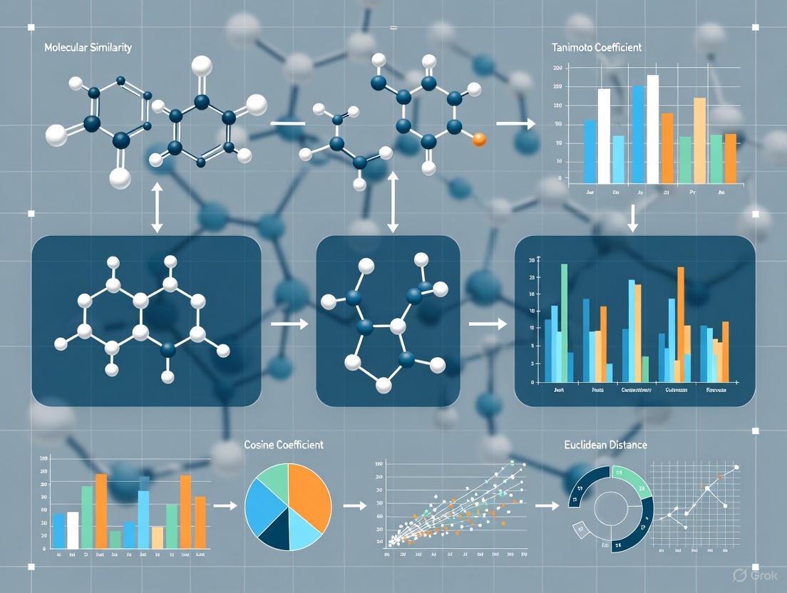
Molecular similarity serves as a cornerstone of modern cheminformatics and drug design, enabling researchers to predict biological activity, navigate chemical space, and identify novel therapeutic candidates [19]. The principle that structurally similar molecules often exhibit similar properties or biological activities underpins many computational approaches in drug discovery [6]. Traditional similarity metrics—including Tanimoto, Jaccard, Dice, and Cosine coefficients—provide the mathematical foundation for quantifying these structural relationships, forming an essential component of the virtual screening toolkit [30]. These metrics, when applied to molecular fingerprints, allow for efficient comparison of chemical structures across large compound databases, facilitating tasks ranging from hit identification to scaffold hopping [24]. This application note details the theoretical basis, practical implementation, and experimental protocols for utilizing these fundamental similarity measures in drug discovery research.
Comparative Analysis of Similarity Metrics
Mathematical Foundations
Traditional similarity metrics operate primarily on binary molecular fingerprints, which encode the presence or absence of structural features as bit vectors [31] [30]. The following table summarizes the key mathematical properties of these fundamental coefficients:
Table 1: Fundamental Similarity and Distance Metrics for Binary Molecular Fingerprints
| Metric Name | Formula for Binary Variables | Minimum | Maximum | Type |
|---|---|---|---|---|
| Tanimoto (Jaccard) | ( T = \frac{x}{y + z - x} ) | 0 | 1 | Similarity |
| Dice (Hodgkin index) | ( D = \frac{2x}{y + z} ) | 0 | 1 | Similarity |
| Cosine (Carbo index) | ( C = \frac{x}{\sqrt{y \cdot z}} ) | 0 | 1 | Similarity |
| Soergel distance | ( S = 1 - T ) | 0 | 1 | Distance |
| Euclidean distance | ( E = \sqrt{(y - x) + (z - x)} ) | 0 | N(_{\alpha}) | Distance |
| Hamming distance | ( H = (y - x) + (z - x) ) | 0 | N(_{\alpha}) | Distance |
Where: x = number of common "on" bits in both fingerprints; y = total "on" bits in fingerprint A; z = total "on" bits in fingerprint B; N(_{\alpha}) = length of the fingerprint [31].
The Tanimoto coefficient (also known as Jaccard coefficient) remains the most widely used similarity measure in cheminformatics, calculating the ratio of shared features to the total number of unique features present in either molecule [31] [30]. Its dominance stems from consistent performance in ranking compounds during structure-activity studies, despite a known bias toward smaller molecules [30].
The Dice coefficient (also called Hodgkin index) similarly measures feature overlap but gives double weight to the common features, making it less sensitive to the absolute size difference between molecules [31] [32].
The Cosine coefficient (Carbo index) measures the angle between two fingerprint vectors in high-dimensional space, effectively capturing directional agreement regardless of vector magnitude [31] [32].
Distance metrics like Soergel, Euclidean, and Hamming quantify dissimilarity rather than similarity. The Soergel distance represents the exact complement of the Tanimoto coefficient (their sum equals 1), while Euclidean and Hamming distances require normalization when converted to similarity scores [31].
Performance Considerations in Virtual Screening
Systematic benchmarking studies have revealed significant performance variations among similarity metrics depending on fingerprint type and biological context. One comprehensive evaluation using chemical-genetic interaction profiles in yeast as a biological activity benchmark found that the optimal pairing of fingerprint encodings and similarity coefficients substantially impacts retrieval rates of functionally similar compounds [30].
Table 2: Benchmarking Performance of Molecular Fingerprints and Similarity Coefficients
| Fingerprint Type | Description | Optimal Similarity Coefficient | Key Application Context |
|---|---|---|---|
| ASP (All-Shortest Paths) | Encodes all shortest topological paths between atoms | Braun-Blanquet | Robust performance across diverse compound collections |
| ECFP (Extended Connectivity Fingerprints) | Circular fingerprints capturing atom environments | Tanimoto, Dice | Structure-activity relationship studies |
| MACCS Keys | 166 structural keys based on functional groups | Tanimoto | Rapid similarity screening |
| RDKit Topological | Daylight-like fingerprint based on molecular paths | Various | General-purpose similarity searching |
The Braun-Blanquet similarity coefficient ((x/max(y,z))), though less commonly discussed, demonstrated superior performance when paired with all-shortest path (ASP) fingerprints in large-scale benchmarking, offering robust retrieval of biologically similar compounds across multiple compound collections [30].
For researchers applying these metrics, a Tanimoto coefficient threshold of 0.85 has historically indicated a high probability of two compounds sharing similar biological activity [31]. However, this threshold is fingerprint-dependent; 0.85 computed from MACCS keys represents different structural similarity than the same value computed from ECFP fingerprints [31].
Experimental Protocols
Protocol 1: Molecular Fingerprint Generation and Similarity Calculation
This protocol describes the standard workflow for generating molecular fingerprints and calculating similarity coefficients using open-source cheminformatics tools.
Figure 1: Workflow for calculating molecular similarity from chemical structures.
Materials and Reagents
Table 3: Essential Research Reagents and Computational Tools
| Item | Function/Description | Example Sources |
|---|---|---|
| RDKit | Open-source cheminformatics toolkit for fingerprint generation | rdkit.org |
| Python 3.7+ | Programming environment for executing analysis | python.org |
| Chemical databases | Sources of molecular structures (e.g., ChEMBL, PubChem) | EMBL-EBI, NIH |
| Molecular structures | Compounds in SMILES format for similarity comparison | In-house libraries, public databases |
Step-by-Step Procedure
Molecular Standardization
- Input molecular structures as Simplified Molecular-Input Line-Entry System (SMILES) strings or structure-data files
- Remove salts and standardize tautomeric forms using RDKit's standardization functions
- Generate canonical SMILES to ensure consistent representation
Fingerprint Generation
- Select appropriate fingerprint type based on application needs:
- ECFP4: 1024-2048 bits, radius 2 for capturing local atom environments
- MACCS Keys: 166 structural keys for rapid screening
- RDKit Topological: Daylight-like fingerprint for general similarity searching
- Generate binary bit vectors using RDKit's fingerprint functions
- Select appropriate fingerprint type based on application needs:
Similarity Coefficient Calculation
- Implement functions to calculate multiple similarity metrics:
- Tanimoto:
T = x / (y + z - x) - Dice:
D = 2x / (y + z) - Cosine:
C = x / sqrt(y * z) - Tversky: Asymmetric similarity with parameters α and β
- Compute similarity matrix for all compound pairs in the dataset
Results Interpretation
- Apply similarity thresholds (Tanimoto > 0.85 for high similarity)
- Generate similarity-property maps to visualize structure-activity relationships
- Identify activity cliffs where high structural similarity corresponds to large activity differences
Protocol 2: Virtual Screening Using Similarity Metrics
This protocol outlines a virtual screening workflow to identify potential bioactive compounds using similarity searching against reference molecules with known activity.
Figure 2: Virtual screening workflow using similarity searching.
Materials and Reagents
Table 4: Virtual Screening Research Resources
| Item | Function/Description | Application Context |
|---|---|---|
| Query compound | Molecule with desired biological activity | Known active from HTS or literature |
| Screening database | Large collection of purchasable or synthesizable compounds | Enamine REAL, ZINC, in-house collections |
- Similarity profiling tools: Software for calculating and visualizing molecular similarity (RDKit, OpenBabel, KNIME)
- High-performance computing: Resources for large-scale similarity calculations across million-compound libraries
Step-by-Step Procedure
Query Compound Preparation
- Select one or more reference compounds with desired biological activity profile
- Generate multiple fingerprint representations (ECFP, MACCS, topological)
- Define relevant similarity thresholds based on fingerprint type and target biology
Database Screening
- Precompute fingerprints for entire screening database to enable rapid similarity searching
- Implement parallel processing for large databases (>1 million compounds)
- Calculate multiple similarity coefficients (Tanimoto, Dice, Cosine) for comprehensive assessment
Hit Identification and Analysis
- Rank database compounds by similarity scores for each metric
- Apply similarity thresholds (typically Tanimoto > 0.6-0.8 for lead identification)
- Select diverse candidates from top-ranking compounds to maintain structural diversity
- Apply scaffold hopping analysis to identify structurally distinct analogs
Experimental Validation
- Procure or synthesize top-ranking compounds for biological testing
- Validate predicted activity through in vitro assays
- Iterate screening process with active compounds as new queries
Applications in Drug Design and Chemical Space Research
Scaffold Hopping and Lead Optimization
Molecular similarity metrics play a crucial role in scaffold hopping—the identification of structurally distinct cores that maintain similar biological activity [24]. Traditional similarity methods utilizing fingerprint-based searches enable researchers to replace problematic molecular scaffolds while preserving key interactions with biological targets [24]. The Tversky similarity metric, with its asymmetric parameters (α and β), offers particular utility in scaffold hopping by allowing differential weighting of features between query and reference molecules [32].
Advanced applications combine multiple similarity metrics to balance structural novelty with maintained bioactivity. For example, a hybrid approach might use Tanimoto similarity to identify initial candidates, followed by Tversky similarity to prioritize compounds with specific feature conservation for synthetic feasibility or intellectual property considerations [32].
Chemical Space Analysis and Diversity Assessment
Similarity metrics provide the foundation for mapping and navigating the vast theoretical chemical space, estimated to contain 10^33 to 10^60 drug-like molecules [33] [34]. The intrinsic similarity (iSIM) framework enables efficient quantification of library diversity through calculation of average pairwise Tanimoto similarity with O(N) computational complexity, bypassing the traditional O(N^2) scaling problem [33].
Recent analyses of evolving chemical libraries (ChEMBL, PubChem, DrugBank) reveal that mere growth in library size does not necessarily translate to increased chemical diversity [33]. By applying similarity metrics to time-stamped database releases, researchers can identify which chemical space regions are expanding and guide future library design toward underrepresented areas.
Integration with Machine Learning Approaches
Traditional similarity metrics are increasingly integrated with modern machine learning frameworks to enhance predictive performance in drug discovery [30]. Quantitative Read-Across Structure-Activity Relationships (RASAR) incorporate similarity descriptors into statistical models, combining the interpretability of similarity-based methods with the predictive power of machine learning [6].
Benchmarking studies demonstrate that support vector machines (SVMs) trained on fingerprint representations can achieve fivefold improvement in biological activity prediction compared to unsupervised similarity searching alone [30]. This hybrid approach leverages the mathematical foundation of traditional similarity metrics while addressing their limitations through learned patterns from bioactivity data.
Traditional similarity metrics—Tanimoto, Dice, Cosine, and related coefficients—continue to provide essential tools for molecular comparison in drug discovery. When properly selected and implemented through standardized protocols, these metrics enable efficient virtual screening, scaffold hopping, and chemical space navigation. While AI-driven approaches represent the frontier of molecular representation, traditional similarity measures remain fundamental components of the cheminformatics toolkit, particularly when combined with machine learning in hybrid frameworks. Their mathematical transparency, computational efficiency, and proven utility across decades of research ensure their continued relevance in addressing the complex challenges of modern drug design.
The pursuit of novel therapeutic compounds relies on the fundamental principle of molecular similarity, which posits that structurally similar molecules often exhibit similar properties [35]. Molecular representation, the process of translating chemical structures into a computer-readable format, serves as the cornerstone for applying artificial intelligence (AI) in drug discovery [24]. Effective representation is a critical prerequisite for training machine learning models to predict molecular behavior, navigate the vast chemical space, and accelerate tasks such as virtual screening and scaffold hopping—the identification of novel core structures that retain biological activity [24].
Traditional representation methods, including molecular descriptors and string-based notations like SMILES, have been widely used but often struggle to capture the intricate relationships between molecular structure and function [24]. The rapid evolution of AI has ushered in a new paradigm of data-driven molecular representation. Among these, Graph Neural Networks (GNNs) and Transformers have emerged as particularly powerful frameworks. GNNs natively model molecules as graphs, with atoms as nodes and bonds as edges, while Transformers, adapted from natural language processing, can process molecular strings or graphs to capture complex, long-range dependencies [24] [36]. This article provides detailed application notes and protocols for leveraging these advanced techniques within the context of molecular similarity and drug design.
From Traditional Descriptors to AI-Driven Embeddings
The journey of molecular representation began with traditional, rule-based methods. The Simplified Molecular-Input Line-Entry System (SMILES) is a prime example, providing a compact string encoding of a molecule's structure [24]. While simple and human-readable, SMILES has inherent limitations; it does not guarantee that similar molecules have similar strings, and it can struggle to represent molecular validity [37]. Molecular fingerprints, such as the Extended Connectivity Fingerprint (ECFP), were another significant advancement, encoding substructural information as fixed-length binary vectors suitable for similarity search and clustering [24].
AI-driven methods represent a fundamental shift from these predefined rules to learned, continuous representations. Deep learning models can extract features directly from data, capturing subtle structural and functional relationships that are difficult to hand-engineer [24]. These approaches can be broadly categorized into those that operate on molecular graphs (GNNs) and those that leverage sequence- or graph-based attention mechanisms (Transformers).
Table 1: Comparison of Molecular Representation Methods
| Method Category | Key Examples | Representation Format | Advantages | Limitations |
|---|---|---|---|---|
| Traditional | SMILES, ECFP, Molecular Descriptors | Strings, Binary Vectors, Numerical Vectors | Computationally efficient, interpretable, good for QSAR [24] | Struggle with complex structure-function relationships, limited exploration of chemical space [24] |
| Graph Neural Networks (GNNs) | GCN, GAT, MPNN, BatmanNet [38] [37] | Graph (Nodes/Edges) | Native representation of molecular topology, powerful for capturing local atomic environments [24] | Can suffer from over-smoothing and over-squashing, limited long-range dependency capture [36] |
| Transformers | Molecular Transformer, Graph Transformer (GT) [35] [39] | Sequences (SMILES) or Graphs with Attention | Superior long-range dependency capture, flexible and customizable architectures [39] [36] | High computational complexity, can underutilize edge information without specific enhancements [40] |
The Rise of Hybrid and Enhanced Architectures
To overcome the limitations of pure GNN or Transformer models, the field has seen a surge in hybrid and enhanced architectures. Graph Transformers (GTs) integrate structural information into the Transformer's self-attention mechanism, allowing it to operate directly on graph-structured data [36]. Furthermore, models like Kolmogorov-Arnold GNNs (KA-GNNs) integrate novel mathematical frameworks to enhance the expressivity and interpretability of traditional GNNs [41]. Another innovative approach is the Bi-branch Masked Graph Transformer Autoencoder (BatmanNet), which uses a self-supervised pre-training strategy to reconstruct masked portions of the molecular graph, effectively learning both local and global information [37].
Quantitative Performance Benchmarking
Evaluating the performance of different models across standardized benchmarks is crucial for assessing their utility in real-world drug discovery tasks. The following tables summarize key quantitative findings from recent studies.
Table 2: Performance Comparison on Molecular Property Prediction Tasks (MAE/RMSE on Quantum Mechanical Datasets) [39]
| Model Architecture | Sterimol B5 (Å) | Sterimol L (Å) | Buried Sterimol B5 (Å) | Binding Energy (kcal/mol) |
|---|---|---|---|---|
| XGBoost (ECFP Baseline) | 0.31 | 0.48 | 0.29 | 4.15 |
| GIN-VN (2D GNN) | 0.25 | 0.41 | 0.24 | 3.82 |
| PaiNN (3D GNN) | 0.22 | 0.38 | 0.21 | 3.65 |
| 2D Graph Transformer (GT) | 0.24 | 0.40 | 0.23 | 3.78 |
| 3D Graph Transformer (GT) | 0.21 | 0.37 | 0.20 | 3.60 |
Table 3: Downstream Task Performance of Pre-trained Models (AUROC/AUPRC) [37]
| Model | BBBP | Tox21 | ClinTox | SIDER |
|---|---|---|---|---|
| Graph Logistic Regression | 0.695 | 0.759 | 0.800 | 0.575 |
| GCN | 0.719 | 0.783 | 0.844 | 0.621 |
| Graph Transformer | 0.735 | 0.795 | 0.865 | 0.635 |
| BatmanNet (Ours) | 0.750 | 0.812 | 0.892 | 0.658 |
The data indicates that 3D-aware models (GNNs and GTs) generally outperform 2D and descriptor-based baselines on tasks involving spatial molecular properties [39]. Furthermore, self-supervised pre-training strategies, as employed by BatmanNet, consistently enhance performance across various molecular property prediction tasks [37].
Application Notes and Detailed Protocols
Protocol 1: Exhaustive Local Chemical Space Exploration with a Regularized Transformer
Application Objective: Systematically generate and evaluate molecules within a defined similarity neighborhood of a lead compound for lead optimization [35].
Background: Standard generative models sample from a vast chemical space but lack explicit control over molecular similarity. This protocol uses a source-target molecular Transformer, regularized with a similarity kernel, to enable exhaustive sampling of a lead compound's "near-neighborhood."
Workflow Diagram:
Step-by-Step Procedure:
Model Training and Preparation:
- Train a source-target molecular Transformer on a large dataset of molecular pairs (e.g., 200 billion pairs from PubChem) [35].
- Incorporate a ranking loss (regularization) term during training. This term aligns the model's Negative Log-Likelihood (NLL) output for a generated molecule with its Tanimoto similarity (using ECFP4 fingerprints) to the source molecule. The loss function is:
L_total = L_NLL + λ * L_rankingwhereL_rankingpenalizes discrepancies between the NLL and similarity rankings [35].
Source Molecule Input:
- Provide the lead compound (source molecule) as a canonicalized SMILES string to the trained Transformer model.
Candidate Generation with Beam Search:
- Use beam search (with a beam width, e.g., 10-100) to generate a set of candidate target molecules. The beam search explores the most probable SMILES token sequences given the source [35].
Similarity-Based Ranking and Filtering:
- For each generated candidate, compute its NLL (a proxy for generation "precedence") and its Tanimoto similarity to the source molecule.
- Rank all generated candidates based on their NLL. Due to the ranking loss during training, a lower NLL will correlate with higher similarity [35].
- Set an NLL threshold to define the boundary of the "near-neighborhood." All molecules with an NLL below this threshold are considered part of the exhaustively sampled neighborhood.
Validation and Canonicalization:
- Validate the chemical validity of all generated SMILES strings using a toolkit like RDKit.
- Canonicalize all valid SMILES to remove duplicates and obtain a standardized representation.
Key Reagents and Computational Tools:
- Software: Python, RDKit, Transformer model code (e.g., PyTorch).
- Model: A pre-trained regularized source-target molecular Transformer.
- Datasets: For training, large-scale molecular pair datasets like PubChem. For evaluation, therapeutic target databases (TTD) [35].
- Similarity Metric: ECFP4 fingerprints with Tanimoto similarity.
Protocol 2: Molecular Property Prediction with a Kolmogorov-Arnold Graph Neural Network (KA-GNN)
Application Objective: Accurately predict molecular properties (e.g., solubility, toxicity) with enhanced accuracy and interpretability.
Background: KA-GNNs integrate Fourier-based Kolmogorov-Arnold network (KAN) modules into the core components of a GNN (node embedding, message passing, readout), replacing standard Multi-Layer Perceptrons (MLPs). This enhances the model's expressivity, parameter efficiency, and ability to highlight chemically meaningful substructures [41].
Workflow Diagram:
Step-by-Step Procedure:
Data Preprocessing and Graph Construction:
- For each molecule in the dataset, generate a graph representation where atoms are nodes and bonds are edges.
- Initialize node features using atomic properties (e.g., atomic number, hybridization, formal charge).
- Initialize edge features using bond properties (e.g., bond type, conjugation).
Model Architecture Configuration (KA-GCN Variant):
- Node Embedding: The initial node embedding is computed by passing the concatenation of its atomic features and the averaged features of its neighboring bonds through a Fourier-based KAN layer [41].
- Message Passing: Implement a Graph Convolutional Network (GCN) layer. However, instead of a standard activation function, update node features using a residual Fourier-KAN module. The message from neighbor j to node i is processed by a learnable Fourier function [41].
- Readout: After multiple message-passing layers, aggregate node features into a single graph-level representation using a readout function (e.g., mean pooling). This graph embedding is then transformed through a final Fourier-KAN layer to produce the property prediction [41].
Model Training:
- Use a standard regression loss (e.g., Mean Squared Error) for property prediction tasks.
- Employ the Adam optimizer and train for a predetermined number of epochs with a defined learning rate scheduler.
Interpretation and Analysis:
- Leverage the inherent interpretability of the KAN modules. The learned Fourier functions on edges can be inspected to understand the importance of specific atomic interactions and substructures for the prediction [41].
Key Reagents and Computational Tools:
- Software: PyTorch or TensorFlow, Deep Graph Library (DGL) or PyTorch Geometric.
- Model: KA-GNN implementation (e.g., KA-GCN or KA-GAT) [41].
- Datasets: Public molecular property benchmarks such as ESOL (solubility), FreeSolv (hydration free energy), or Tox21 (toxicity) [38].
Protocol 3: Self-Supervised Pre-training with BatmanNet for Data-Efficient Learning
Application Objective: Learn powerful, general-purpose molecular representations from unlabeled data to boost performance on downstream tasks with limited labeled examples.
Background: BatmanNet is a bi-branch masked graph transformer autoencoder designed for self-supervised learning. It masks a high proportion (e.g., 40%) of nodes and edges and learns to reconstruct them, forcing the model to capture rich structural and semantic information [37].
Workflow Diagram:
Step-by-Step Procedure:
Pre-training Data Curation:
- Assemble a large dataset of unlabeled molecules from sources like PubChem or ZINC. BatmanNet was trained on approximately 10 million molecules [37].
Self-Supervised Pre-training:
- For each molecular graph in a batch, randomly mask 40% of its nodes and 40% of its edges [37].
- The encoder of BatmanNet, a transformer-style architecture with integrated GNN-Attention blocks, processes only the visible, unmasked subset of the graph.
- The lightweight, asymmetric decoder takes the encoder's output and the mask tokens and attempts to reconstruct the original, unmasked graph.
- The model is trained by minimizing the reconstruction loss, which is a composite loss for predicting the identities of masked nodes and the existence/types of masked edges [37].
Transfer Learning to Downstream Tasks:
- After pre-training, discard the decoder.
- The pre-trained encoder is used as a feature extractor for downstream tasks. It can be fine-tuned on smaller, labeled datasets for tasks like property prediction, drug-drug interaction, or drug-target interaction prediction [37].
Key Reagents and Computational Tools:
- Software: Python, PyTorch, RDKit.
- Model: BatmanNet implementation.
- Datasets: Large-scale unlabeled datasets (e.g., PubChem) for pre-training; specific benchmarks (e.g., BBBP, HIV, DDI datasets) for downstream evaluation [37].
Table 4: Key Computational Tools and Datasets for AI-Driven Molecular Representation
| Category | Item | Description and Function |
|---|---|---|
| Software & Libraries | RDKit | Open-source cheminformatics toolkit used for molecule manipulation, fingerprint generation, and descriptor calculation. |
| PyTorch Geometric / DGL | Python libraries that provide a wide range of GNN models and utilities, simplifying the implementation of graph-based deep learning. | |
| Transformers Library (Hugging Face) | Provides a vast collection of pre-trained Transformer models, with a growing ecosystem for chemical and biological applications. | |
| GNN Architectures | GCN, GAT, GIN | Foundational GNN architectures that serve as strong baselines and building blocks for more complex models [38]. |
| KA-GNN | A GNN variant using Kolmogorov-Arnold Networks for enhanced accuracy and interpretability in property prediction [41]. | |
| Transformer Architectures | Graph Transformer (GT) | A Transformer adapted for graph data, often using structural positional encoding or structure-aware attention [39] [36]. |
| Molecular Transformer | A sequence-based Transformer operating on SMILES, commonly used for molecular translation and optimization tasks [35]. | |
| Benchmark Datasets | MoleculeNet | A curated collection of molecular property prediction datasets (e.g., ESOL, FreeSolv, BBBP, Tox21) for standardized benchmarking [38]. |
| OGB (Open Graph Benchmark) | Provides large-scale, diverse, and realistic graph datasets for benchmarking graph ML models, including molecular graphs [39]. | |
| Pre-trained Models | BatmanNet | A self-supervised, pre-trained graph model that can be fine-tuned for various downstream tasks with limited labeled data [37]. |
The adoption of GNNs and Transformers for molecular representation has fundamentally transformed the landscape of computer-aided drug discovery. These AI-driven methods provide a powerful means to navigate chemical space based on learned, data-driven similarity measures that surpass the capabilities of traditional fingerprints. The protocols outlined for exhaustive chemical space exploration, property prediction with interpretable models, and self-supervised pre-training provide a practical roadmap for researchers to integrate these advanced techniques into their workflows. As these architectures continue to evolve—through better integration of 3D information, more efficient attention mechanisms, and novel mathematical frameworks—their capacity to capture the intricate language of chemistry will only deepen, further accelerating the rational design of novel therapeutics.
Scaffold hopping has emerged as a critical strategy in medicinal chemistry for generating novel, patentable drug candidates while preserving biological activity. This approach systematically modifies the core molecular structure of known bioactive compounds to explore uncharted chemical space, addressing challenges such as intellectual property constraints, toxicity, and poor pharmacokinetic profiles. By leveraging advanced molecular similarity measures including Tanimoto coefficients, electron shape comparisons, and pharmacophore matching, researchers can identify structurally diverse compounds with similar biological functions. Recent computational advances have dramatically accelerated scaffold hopping, enabling more efficient navigation of the vast chemical space and opening new frontiers in drug discovery.
Scaffold hopping, first coined by Schneider and colleagues in 1999, represents a cornerstone strategy in modern drug discovery [42]. This approach aims to identify compounds with different core structures (scaffolds) that maintain similar biological activities or property profiles as their parent molecules [24]. The fundamental premise relies on the concept of molecular similarity—the principle that structurally different compounds can share key physicochemical properties that enable interaction with specific biological targets.
The strategic importance of scaffold hopping extends across multiple dimensions of drug development. First, it enables circumvention of existing intellectual property barriers by creating novel chemotypes with distinct patent landscapes [43]. Second, it addresses limitations of lead compounds, including metabolic instability, toxicity issues, and suboptimal physicochemical properties [42]. Third, it facilitates exploration of previously inaccessible chemical space, potentially revealing compounds with enhanced efficacy and safety profiles [24]. Market success stories including Vadadustat, Bosutinib, Sorafenib, and Nirmatrelvir demonstrate the tangible impact of scaffold hopping in delivering clinically approved therapeutics [42].
The theoretical foundation of scaffold hopping rests upon molecular similarity principles, which posit that biological activity depends more on specific physicochemical properties and spatial arrangements of functional groups than on the underlying molecular framework itself. By quantifying and leveraging these similarity measures, researchers can systematically navigate chemical space to identify novel scaffolds while preserving critical pharmacophoric elements.
Molecular Similarity: The Theoretical Framework
Fundamental Similarity Metrics
Effective scaffold hopping relies on robust molecular similarity measures that capture essential features for maintaining biological activity:
Tanimoto Similarity: Based on molecular fingerprints, this metric quantifies structural overlap using binary vectors representing molecular substructures. It provides a rapid, two-dimensional similarity assessment with values ranging from 0 (no similarity) to 1 (identical structures) [42]. While computationally efficient, it may overlook critical three-dimensional features essential for biological activity.
Electron Shape Similarity: This approach, implemented through tools like ElectroShape, extends beyond structural resemblance to incorporate three-dimensional electron density distributions and charge characteristics [42]. By capturing electrostatic complementarity to biological targets, it offers enhanced prediction of conserved activity across scaffold transitions.
Pharmacophore Similarity: This metric focuses on conserved spatial arrangements of functional groups essential for molecular recognition and biological activity, including hydrogen bond donors/acceptors, hydrophobic regions, and charged centers [24]. Pharmacophore-based scaffold hopping strategically preserves these critical interaction elements while modifying the intervening molecular framework.
Classification of Scaffold Hops
Scaffold hopping maneuvers can be systematically categorized into distinct classes based on structural modification strategy:
Table: Classification of Scaffold Hopping Approaches
| Hop Category | Structural Modification | Similarity Preservation | Typical Applications |
|---|---|---|---|
| Heterocyclic Replacement (1°) | Swapping carbon/heteroatoms in core rings | Electronic distribution, shape complementarity | Bioisosteric replacement, property optimization |
| Ring Opening/Closing (2°) | Converting cyclic systems to acyclic or vice versa | Pharmacophore alignment, conformational flexibility | Peptidomimetics, solubility enhancement |
| Peptide Mimicry | Replacing peptide backbone with non-peptide scaffolds | Spatial positioning of key functional groups | Protease inhibitors, PPI stabilizers |
| Topology-Based | Altering core connectivity while maintaining overall shape | Molecular volume, surface characteristics | Patent expansion, scaffold diversification |
This classification, initially proposed by Sun et al., provides a systematic framework for understanding and designing scaffold hopping strategies with increasing degrees of structural departure from original compounds [24].
Computational Framework: ChemBounce Protocol
ChemBounce represents an open-source computational framework specifically designed for scaffold hopping applications, leveraging a curated library of over 3.2 million synthesis-validated fragments derived from the ChEMBL database [42]. The platform integrates multiple similarity metrics to balance structural novelty with conserved biological activity potential.
Detailed Experimental Protocol
Step 1: Input Preparation and Validation
- Input Format: Prepare the query molecule as a valid SMILES string without salts or multiple components separated by "." notation [42].
- Validation: Confirm SMILES syntax including balanced brackets, valid atomic symbols, correct valence assignments, and proper ring closure numbering.
- Command Implementation:
Step 2: Molecular Fragmentation
- Apply the HierS algorithm from ScaffoldGraph to systematically decompose the input molecule into ring systems, side chains, and linkers [42].
- Generate basis scaffolds by removing all linkers and side chains, preserving only ring systems.
- Generate superscaffolds that retain linker connectivity between ring systems.
- Execute recursive ring removal to generate all possible scaffold combinations until no smaller scaffolds exist.
Step 3: Scaffold Library Querying
- Access the curated ChEMBL-derived scaffold library containing 3,231,556 unique scaffolds [42].
- Calculate Tanimoto similarity between query scaffold and all library entries based on molecular fingerprints.
- Apply similarity threshold (default: 0.5) to identify candidate replacement scaffolds.
- For advanced applications, implement custom scaffold libraries using the
--replace_scaffold_filesoption.
Step 4: Scaffold Replacement and Molecule Generation
- Replace the query scaffold with candidate scaffolds from the similarity-filtered library.
- Preserve critical substructures using the
--core_smilesoption to maintain essential pharmacophoric elements. - Generate novel molecular structures with the replaced scaffolds while maintaining original side-chain connectivity.
Step 5: Similarity Rescreening and Output
- Calculate electron shape similarity between generated structures and original input using ElectroShape implementation in the Open Drug Discovery Toolkit (ODDT) [42].
- Apply combined similarity threshold (Tanimoto + electron shape) to filter generated compounds.
- Export final candidate structures to specified output directory with similarity metrics and structural annotations.
Parameter Optimization and Validation
Performance validation across diverse molecule types reveals critical parameter considerations:
Table: ChemBounce Performance Metrics Across Compound Classes
| Compound Type | Example | Molecular Weight Range (Da) | Processing Time | Optimal Similarity Threshold |
|---|---|---|---|---|
| Small Molecules | Celecoxib, Rimonabant | 315-450 | 4-15 seconds | 0.5-0.6 |
| Peptides | Kyprolis, Trofinetide | 450-800 | 2-5 minutes | 0.4-0.5 |
| Macrocyclic Compounds | Pasireotide, Motixafortide | 800-1500 | 5-12 minutes | 0.3-0.4 |
| Complex Molecules | Venetoclax, Lapatinib | 450-900 | 8-21 minutes | 0.5-0.7 |
Comparative analyses against commercial platforms (Schrödinger's Ligand-Based Core Hopping, BioSolveIT's FTrees, SpaceMACS, and SpaceLight) demonstrate that ChemBounce generates structures with lower synthetic accessibility scores (SAscore) and improved quantitative estimate of drug-likeness (QED) values [42].
Advanced Applications and Case Studies
Tuberculosis Drug Discovery
Scaffold hopping has demonstrated particular utility in addressing drug-resistant Mycobacterium tuberculosis strains through targeting of key pathways including energy metabolism, cell wall synthesis, and proteasome function [44]. The approach has yielded compounds with improved pharmacokinetic profiles, enhanced efficacy, and reduced toxicity while circumventing existing resistance mechanisms.
Molecular Glue Development
Recent work on 14-3-3/ERα complex stabilization exemplifies the power of scaffold hopping in molecular glue development [45]. Using the AnchorQuery platform to screen a 31-million compound library of synthetically accessible multi-component reaction products, researchers identified novel imidazo[1,2-a]pyridine scaffolds that effectively stabilized the protein-protein interaction.
Experimental Protocol: Pharmacophore-Based Scaffold Hopping
Step 1: Anchor Identification
- Analyze crystal structure of bound ligand (PDB: 8ALW) to identify deeply buried "anchor" motif (p-chloro-phenyl ring forming halogen bond with K122) [45].
Step 2: Pharmacophore Definition
- Define three-point pharmacophore incorporating key ligand-protein interactions:
- Hydrogen bond acceptor matching tetrahydropyrane oxygen
- Hydrophobic feature matching aliphatic ring interactions
- Hydrogen bond donor matching aniline nitrogen
Step 3: Library Screening
- Screen 31+ million compound library using RMSD fit ranking with molecular weight filter (<400 Da).
- Identify top-ranking imidazo[1,2-a]pyridine scaffolds from Groebke-Blackburn-Bienaymé multi-component reaction.
Step 4: Complex Formation and Validation
- Synthesize lead candidates using GBB-3CR with aldehydes, 2-aminopyridines, and isocyanides.
- Determine co-crystal structures of ternary complexes (glue + 14-3-3 + phospho-ERα peptide).
- Validate cellular stabilization using NanoBRET assay with full-length proteins in live cells.
Reinforcement Learning Approaches
The RuSH (Reinforcement Learning for Unconstrained Scaffold Hopping) framework demonstrates the integration of generative AI with scaffold hopping [46]. Unlike traditional constrained generation, RuSH employs reinforcement learning to steer full-molecule generation toward high three-dimensional and pharmacophore similarity to reference molecules while minimizing scaffold similarity, enabling more comprehensive exploration of chemical space.
Research Reagents and Computational Tools
Table: Essential Research Reagents and Computational Platforms for Scaffold Hopping
| Tool/Resource | Type | Primary Function | Access |
|---|---|---|---|
| ChemBounce | Computational Framework | Scaffold identification and replacement with similarity filtering | Open-source (GitHub) [42] |
| ScaffoldGraph | Python Library | Molecular fragmentation and scaffold analysis | Open-source |
| ChEMBL Database | Scaffold Library | 3.2+ million curated, synthesis-validated scaffolds | Public database [42] |
| AnchorQuery | Pharmacophore Platform | MCR-based scaffold screening and design | Freely accessible [45] |
| ElectroShape/ODDT | Similarity Tool | Electron shape similarity calculations | Open-source Python library [42] |
| BioSolveIT infiniSee | Chemical Space Platform | Navigation of trillion-compound chemical spaces | Commercial [10] |
| SeeSAR | Structure-Based Design | Interactive structure-based compound optimization | Commercial [10] |
| Enamine REAL Space | Compound Library | Commercially available compounds for synthesis | Screening library [10] |
Scaffold hopping represents a powerful strategy for navigating the complex landscape of chemical space in drug discovery. By leveraging sophisticated molecular similarity measures including Tanimoto coefficients, electron shape comparisons, and pharmacophore matching, researchers can systematically generate novel chemotypes with conserved biological activity. The integration of computational frameworks like ChemBounce with advanced experimental validation creates a robust pipeline for scaffold exploration and optimization. As molecular representation methods continue to evolve, particularly with advances in AI-driven approaches, scaffold hopping will undoubtedly remain an essential component of the drug discovery toolkit, enabling more efficient exploration of chemical space and acceleration of therapeutic development.
Drug repurposing represents a strategic approach to identify new therapeutic uses for existing drugs, offering the potential to reduce development timelines and costs while leveraging existing safety and pharmacokinetic data [47] [48]. Within the broader context of molecular similarity measures in drug design, the fundamental hypothesis is that drugs sharing clinical indications induce similar changes in gene expression profiles, and that these transcriptional signatures can serve as a proxy for predicting new therapeutic applications [49] [47]. This application note details protocols for leveraging transcriptional and clinical profile similarity to systematically identify drug repurposing candidates, framed within the conceptual framework of the biologically relevant chemical space (BioReCS) [4].
Core Concepts and Rationale
The methodological foundation rests on two complementary principles derived from the analysis of genome-wide gene expression data. First, the "reversal of disease signature" principle posits that a drug capable of inducing a gene expression signature negatively correlated with a disease signature may counteract the disease phenotype [47]. Second, the "drug-drug similarity" principle suggests that drugs eliciting highly similar transcriptional responses, even with different chemical structures, may share mechanisms of action and thus therapeutic indications [49] [47]. Recent evidence strongly supports the hypothesis that drugs known to share a clinical indication induce significantly more similar gene expression changes compared to random drug pairs, providing a validated foundation for repurposing algorithms [49].
The following table summarizes essential data resources and their roles in transcriptional profile-based drug repurposing.
Table 1: Key Research Resources for Transcriptional Profile-Based Drug Repurposing
| Resource Name | Type | Primary Function | Key Features/Applications |
|---|---|---|---|
| LINCS L1000 [49] [50] | Transcriptional Database | Profiles gene expression changes for thousands of compounds across cell lines. | Provides Level 5 data (drug gene signatures) and Transcriptional Activity Score (TAS). |
| Drug Repurposing Hub [49] | Curated Drug Indication Database | Catalog of known drug-indication pairs. | Serves as a gold-standard reference for training and validating predictive models. |
| cMap (Connectivity Map) [47] | Transcriptional Database & Tool | Database of expression profiles and pattern-matching tool. | Enables signature reversion analysis via Gene Set Enrichment Analysis (GSEA). |
| DrSim [50] | Computational Framework | Learning-based framework for inferring transcriptional similarity. | Addresses high dimensionality and noise in high-throughput data for improved performance. |
| DrugBank [48] | Drug & Target Database | Provides drug, target, and mechanism of action information. | Used for constructing drug-gene-disease networks and interpreting predictions. |
| AACT Database [49] | Clinical Trials Database | Registry of clinical studies from ClinicalTrials.gov. | Provides independent data for validating model predictions on experimental drug uses. |
Quantitative Comparison of Similarity Metrics
The choice of similarity metric is critical for accurate prediction. The following table compares the performance of different metrics and data processing strategies as evidenced by recent research.
Table 2: Performance Comparison of Similarity Metrics and Data Filters in Drug Indication Prediction
| Metric / Filter | Performance / Effect | Context and Notes |
|---|---|---|
| Spearman Correlation [49] | p = 7.71e-38 | Rank sum test for shared indication drug pairs vs. non-shared pairs; outperformed Connectivity Score. |
| Connectivity Score (CMap) [49] | p = 5.2e-6 | Rank sum test for shared indication drug pairs vs. non-shared pairs. |
| Transcriptional Activity Score (TAS) Filter [49] | Varies with threshold | Filtering signatures by TAS (e.g., 0.2 to 0.5) improves prediction AUC but reduces drug coverage. |
| Ensemble Model (3 cell lines) [49] | AUC = 0.708 | Validated on independent clinical trials data from AACT database, demonstrating generalizability. |
| DrSim (Learning-based) [50] | Outperforms existing methods | Evaluated on public in vitro and in vivo datasets for drug annotation and repositioning. |
Experimental Protocols
Protocol: Drug-Drug Similarity-Based Repurposing
This protocol uses the similarity in transcriptional responses between a candidate drug and known treatments for a disease to predict new indications [49].
Workflow Overview:
Step-by-Step Procedure:
- Data Retrieval: Download Level 5 LINCS L1000 data, which contains drug-induced gene expression signatures (changes across 978 landmark genes) and associated Transcriptional Activity Scores (TAS) for the desired cell lines (e.g., MCF7, A375, PC3) [49].
- Signature Pre-processing: For each drug, select the single gene expression signature (from among multiple dosages and time points) with the highest TAS value to represent its effects. This mitigates redundancy and selects the most robust signature [49].
- Similarity Calculation: For all pairs of drug signatures from the same cell line, compute a similarity metric. Spearman correlation is recommended based on its superior performance [49]. This generates a drug-drug similarity matrix.
- Similarity to Known Treatments: For a target disease, retrieve all drugs known to treat it from the Drug Repurposing Hub. For a candidate drug, its similarity score for the disease is the maximum Spearman correlation between its signature and the signature of any known treatment for that disease [49].
- Model Training and Prediction: Use the maximum similarity score as a feature in a logistic regression model to predict the probability that the candidate drug treats the indication. For improved robustness, train individual models on data from different cell lines and combine them into an ensemble model [49].
- Validation: Evaluate the final model's performance on an independent dataset, such as drug-indication pairs sourced from the AACT database of ongoing clinical trials, by calculating the Area Under the receiver operating characteristic Curve (AUC) [49].
Protocol: Signature Reversion-Based Repurposing
This protocol identifies drugs that can reverse a disease's gene expression signature, based on the assumption that this transcriptional reversal may correlate with phenotypic reversion [47].
Conceptual Workflow:
Step-by-Step Procedure:
- Define Disease Signature: Obtain or generate a gene expression signature for the disease of interest. This is typically a set of genes found to be differentially expressed (up- and down-regulated) when comparing diseased versus healthy tissue samples [47].
- Access Drug Signatures: Access a database of drug-induced gene expression signatures, such as the original Connectivity Map (cMap) or the LINCS L1000 database [47].
- Signature Matching: Use a pattern-matching tool, such as the Gene Set Enrichment Analysis (GSEA)-based method provided by the cMap platform, to query the disease signature against the database of drug signatures [47].
- Identify Reverting Drugs: Prioritize drugs whose gene expression signatures are significantly negatively correlated with the disease signature. This indicates that the drug effect is opposite to the disease effect at the transcriptional level [47].
Advanced and Integrated Methodologies
Network-Based Community Detection
This methodology projects complex drug-gene-disease relationships into a drug-drug similarity network to uncover communities of drugs with shared properties, which can be labeled to generate repurposing hints [48].
Integrated Repurposing Pipeline:
Procedure:
- Network Construction: Construct a tripartite network integrating data from sources like DrugBank (drug-target) and DisGeNET (gene-disease) [48].
- Network Projection: Project this heterogeneous network into a homogeneous drug-drug similarity network, where link strength is based on shared gene or disease associations [48].
- Community Detection: Apply unsupervised clustering algorithms to identify communities (clusters) of drugs within this network [48].
- Community Labeling: Automatically label each detected community using Anatomical Therapeutic Chemical (ATC) codes. Drugs within a community that do not share the community's dominant ATC code are flagged as potential repurposing candidates [48].
- Validation and Prioritization: Validate hints through automated literature searches and prioritize candidates for further investigation using targeted molecular docking on targets associated with the community's ATC label [48].
Machine Learning-Enhanced Similarity
Traditional unsupervised similarity metrics (e.g., Spearman) can suffer from the high dimensionality and noise inherent in transcriptional data. The DrSim framework addresses this by using a metric learning approach to automatically infer a robust, task-specific similarity measure from the data, which has been shown to outperform traditional methods in drug annotation and repositioning tasks [50].
Virtual screening has become a cornerstone of modern drug discovery, serving as a rapid and cost-effective method to narrow down vast chemical libraries to a manageable number of promising hits worthy of experimental validation [51]. The exponential growth of commercially available chemical space, which now encompasses tens of billions of synthesizable compounds, presents both unprecedented opportunities and significant computational challenges for researchers [51]. Efficiently navigating these ultra-large libraries requires sophisticated approaches that balance computational expense with predictive accuracy.
At its core, virtual screening operates on the molecular similarity principle, which posits that structurally similar molecules are likely to exhibit similar biological activities [19] [6]. This principle has become particularly evident in the current data-intensive era of chemical research, with similarity measures serving as the backbone of many machine learning procedures [19] [52]. The concept of molecular similarity has evolved from its original focus on structural resemblance to encompass broader contexts including physicochemical properties, biological activity profiles, and binding interactions [6].
Virtual screening typically serves two distinct purposes in drug discovery pipelines: library enrichment, where very large numbers of diverse compounds are screened to identify a subset with a higher proportion of actives; and compound design, involving detailed analysis of smaller series to guide optimization toward improved potency and drug-like properties [51]. This application note provides a comprehensive overview of current methodologies, protocols, and practical considerations for efficiently mining ultra-large chemical libraries, with particular emphasis on the central role of molecular similarity in structuring chemical space and enabling predictive modeling.
Molecular Similarity: The Theoretical Framework
Foundations of Molecular Similarity
The concept of molecular similarity represents one of the most fundamental abstractions in chemical research, providing a theoretical foundation for understanding and predicting chemical behavior [6]. According to the similarity principle, similar compounds—those sharing molecular structure characteristics—should exhibit similar properties and biological activities. However, this principle encounters limitations in cases of the similarity paradox and activity cliffs, where small structural modifications result in dramatic changes in biological activity [6].
Molecular similarity can be quantified through various descriptors and fingerprints that encode chemical structural information in numerical formats amenable to computational analysis [6]. These representations range from simplified structural keys to complex quantum mechanical descriptions, with the choice of representation heavily influencing the outcome and interpretation of virtual screening campaigns.
Chemical Representations and Descriptors
The representation of chemical structures has evolved significantly from graph-based understandings of organic structure first introduced approximately 150 years ago [6]. Current approaches include:
- Molecular graphs: Describe molecules by their constituent atoms and bonds, enabling computation of structural motifs and fingerprints while requiring reasonable computational resources [6].
- Quantum mechanical descriptions: Offer the most precise representation through solutions to Schrödinger equations but remain computationally prohibitive for large libraries [6].
- Density functional theory (DFT): Provides a balance between accuracy and computational feasibility for predicting chemical reactivity and toxicant-target interactions [6].
- Fingerprints and structural keys: Encode presence or absence of specific structural features as bit strings, enabling rapid similarity comparisons between molecules [6].
Table 1: Molecular Representation Methods and Their Applications in Virtual Screening
| Representation Type | Computational Cost | Primary Applications | Key Considerations |
|---|---|---|---|
| 2D Fingerprints | Low | Initial library filtering, scaffold hopping | Fast but may miss stereochemistry |
| 3D Pharmacophores | Medium | Structure-based screening, binding mode prediction | Requires conformation generation |
| Molecular Graphs | Medium | QSAR modeling, similarity searching | Balances detail with computational efficiency |
| Quantum Mechanical | Very High | Reactivity prediction, electronic properties | Limited to small compound sets |
| Field-based | High | Molecular alignment, scaffold hopping | Captures electrostatic and shape properties |
Virtual Screening Methodologies
Virtual screening methods fall broadly into two complementary categories: ligand-based and structure-based approaches, each with distinct strengths, limitations, and optimal application domains [51].
Ligand-Based Virtual Screening
Ligand-based virtual screening does not require a target protein structure, instead leveraging known active ligands to identify hits that show similar structural or pharmacophoric features [51]. These approaches excel at pattern recognition and generalization across diverse chemistries, making them particularly valuable during early discovery stages for prioritizing large chemical libraries, especially when no protein structure is available [51].
For screening ultra-large chemical spaces containing tens of billions of compounds, methods including infiniSee (BioSolveIT) and exaScreen (Pharmacelera) enable efficient assessment of pharmacophoric similarities between library compounds and known active ligands [51]. These technologies trade off speed in exploring vast spaces with sensitivity and precision, focusing on identifying potential to form critical interaction types rather than detailed binding predictions.
For smaller libraries (up to millions of compounds), advanced ligand-based methods like eSim (Optibrium), ROCS (OpenEye Scientific), and FieldAlign (Cresset) perform detailed conformational analysis by superimposing 3D structures to maximize similarity across pharmacophoric features such as shape, electrostatics, and hydrogen bonding interactions [51]. Quantitative Surface-field Analysis (QuanSA) extends this approach by constructing physically interpretable binding-site models based on ligand structure and affinity data using multiple-instance machine learning, providing predictions for both ligand binding pose and quantitative affinity across chemically diverse compounds [51].
Structure-Based Virtual Screening
Structure-based virtual screening utilizes target protein structural information, typically obtained through experimental methods (X-ray crystallography, cryo-electron microscopy) or computational approaches (homology modeling) [51]. These methods provide insights into atomic-level interactions including hydrogen bonds and hydrophobic contacts, often yielding better enrichment for virtual libraries by incorporating explicit information about binding pocket shape and volume [51].
The most common structure-based approach involves molecular docking, where compounds are computationally positioned and scored within known binding pockets [53] [51]. While numerous docking methods excel at placing ligands into binding sites in reasonable orientations, accurately scoring and ranking these poses remains challenging [51]. State-of-the-art affinity prediction methods like Free Energy Perturbation (FEP) calculations offer improved accuracy but are computationally demanding and typically limited to small structural modifications around known reference compounds [51].
The emergence of AlphaFold (Google DeepMind) has significantly expanded the availability of protein structures, though important quality considerations remain regarding their reliability in docking performance [51]. AlphaFold models typically predict single static conformations, potentially missing ligand-induced conformational changes, and may struggle with side chain positioning critical for accurate docking results [51]. Recent co-folding methods like Boltz-2 (MIT and Recursion) and AlphaFold3 that generate ligand-bound protein structures show promise but questions remain about their generalizability, particularly for predicting allosteric binding sites [51].
Hybrid Screening Approaches
Evidence strongly supports hybrid approaches that combine atomic-level insights from structure-based methods with pattern recognition capabilities of ligand-based approaches [51]. These integrated strategies can outperform individual methods by reducing prediction errors and increasing confidence in hit identification through two primary frameworks:
Sequential Integration
This approach first employs rapid ligand-based filtering of large compound libraries, followed by structure-based refinement of the most promising subset [51]. For example, an initial ligand-based screen can identify novel scaffolds early, offering chemically diverse starting points that can then be analyzed through docking experiments to confirm binding interactions [51]. This strategy conserves computationally expensive calculations for compounds likely to succeed, increasing efficiency while improving precision over single-method approaches.
Parallel Screening
Parallel screening involves running ligand- and structure-based screening independently but simultaneously on the same compound library, with each method generating its own ranking [51]. Results can be compared or combined using:
- Parallel scoring: Selecting top candidates from both approaches without requiring consensus, increasing likelihood of recovering potential actives while mitigating limitations inherent in each approach [51].
- Hybrid (consensus) scoring: Creating a unified ranking through multiplicative or averaging strategies that favor compounds ranking highly across both methods, reducing candidate numbers while increasing confidence in selecting true positives [51].
Application Notes & Protocols
Protocol for Automated Virtual Screening Pipeline
The following protocol outlines a comprehensive workflow for automated virtual screening of ultra-large chemical libraries, integrating both ligand- and structure-based methods for optimal efficiency and predictive accuracy [54] [51].
Diagram 1: VS workflow for ultra-large libraries
Library Generation and Preparation
- Objective: Compile and prepare ultra-large chemical library for virtual screening
- Input: Commercial catalogues (e.g., ZINC, Enamine), corporate collections, virtual combinatorial libraries
- Processing Steps:
- Standardization: Remove duplicates, standardize tautomers, normalize charges
- Descriptor Calculation: Generate molecular fingerprints, physicochemical descriptors
- Drug-likeness Filtering: Apply Ro5, PAINS, and other structural alerts
- Conformational Sampling: Generate representative 3D conformations for each compound
- Output: Curated, search-ready chemical library
Ligand-Based Screening Protocol
- Objective: Rapidly filter ultra-large library using known active ligands as reference
- Input: Curated chemical library, known active compounds (10-50 structures recommended)
- Methodology:
- Similarity Searching: Calculate 2D structural similarity using Tanimoto coefficient on ECFP4 fingerprints
- Pharmacophore Screening: Align compounds to 3D pharmacophore models derived from active ligands
- Shape-Based Screening: Use ROCS or similar tools for molecular shape comparison
- Machine Learning Models: Train similarity-based classification models (e.g., SVM, Random Forest)
- Parameters:
- Similarity threshold: ≥0.7 Tanimoto coefficient for ECFP4
- Pharmacophore fit value: ≥0.8 for critical features
- Shape similarity: ≥0.7 Tanimoto-Combo score
- Output: Top 1-5% of library ranked by ligand-based criteria
Structure-Based Screening Protocol
- Objective: Evaluate compounds using target protein structure information
- Input: Protein structure (experimental or modeled), filtered compound library from ligand-based step
- Methodology:
- Binding Site Preparation: Define binding pocket, add hydrogens, optimize side chain orientations
- Molecular Docking: Use high-throughput docking (e.g., FRED, AutoDock Vina) to pose compounds
- Scoring Function Application: Rank poses using empirical, force field, or knowledge-based scoring
- Ensemble Docking (Optional): Dock against multiple receptor conformations if available
- Parameters:
- Docking exhaustiveness: Standard vs. high precision settings
- Pose clustering: RMSD threshold of 2.0Å for pose selection
- Consensus scoring: Combine multiple scoring functions for improved ranking
- Output: Top 0.1-1% of library ranked by structure-based criteria
Consensus Scoring and Hit Prioritization
- Objective: Integrate results from multiple screening approaches to identify high-confidence hits
- Input: Ranked lists from ligand-based and structure-based screening
- Methodology:
- Rank Fusion: Apply rank aggregation methods (Borda count, RRF)
- Score Normalization: Z-score or min-max normalization across different scoring functions
- Multi-Parameter Optimization: Incorporate additional criteria (drug-likeness, synthetic accessibility)
- Visual Inspection: Manual review of top-ranking compound interactions
- Output: Final hit list (50-500 compounds) for experimental validation
Quantitative Performance Assessment
Recent comparative studies have systematically evaluated virtual screening methodologies using statistical correlation metrics and error-based measures [53]. Key findings include:
Table 2: Performance Comparison of Virtual Screening Methodologies for Urease Inhibitors [53]
| Screening Method | Spearman Correlation (ρ) | Pearson Correlation (r) | Mean Absolute Error | Key Applications |
|---|---|---|---|---|
| MM-GBSA | 0.72 | 0.68 | 1.24 kcal/mol | High-accuracy ranking |
| Ensemble Docking | 0.69 | 0.65 | 1.31 kcal/mol | Handling receptor flexibility |
| Induced-Fit Docking | 0.64 | 0.61 | 1.42 kcal/mol | Accounting for side chain movements |
| QPLD | 0.61 | 0.58 | 1.51 kcal/mol | Systems with metal ions |
| Standard Docking | 0.58 | 0.54 | 1.63 kcal/mol | Initial library screening |
The study also investigated the influence of data fusion techniques and found that while increasing the number of poses generally reduces predictive accuracy, the minimum fusion approach remains robust across all conditions [53]. Comparisons between IC50 and pIC50 as experimental reference values revealed that pIC50 provides higher Pearson correlations, reinforcing its suitability for affinity prediction [53].
The Scientist's Toolkit: Essential Research Reagents
Table 3: Key Software Tools and Platforms for Virtual Screening
| Tool/Platform | Type | Primary Function | Application Context |
|---|---|---|---|
| infiniSee (BioSolveIT) | Ligand-based | Ultra-large library screening | Pharmacophoric similarity searching in billion+ compound spaces |
| exaScreen (Pharmacelera) | Ligand-based | High-throughput screening | Pattern recognition in diverse chemical libraries |
| eSim (Optibrium) | Ligand-based | 3D similarity assessment | Automated identification of similarity criteria for compound ranking |
| ROCS (OpenEye) | Ligand-based | Shape-based screening | Molecular overlay and shape comparison |
| QuanSA (Optibrium) | Ligand-based | Quantitative affinity prediction | Binding-site modeling using multiple-instance machine learning |
| AutoDock Vina | Structure-based | Molecular docking | Protein-ligand interaction analysis and pose prediction |
| Schrödinger Suite | Structure-based | Comprehensive drug discovery | Docking, MM-GBSA, and FEP calculations |
| AlphaFold (DeepMind) | Structure-based | Protein structure prediction | Generating target models when experimental structures unavailable |
| FEP+ (Schrödinger) | Structure-based | Free energy calculations | High-accuracy affinity prediction for lead optimization |
Advanced Applications and Case Studies
RASAR: Integrating Read-Across with QSAR
Recent advances have merged read-across (RA) with quantitative structure-activity relationship (QSAR) principles to develop read-across structure-activity relationship (RASAR) models [6]. This approach uses statistical and machine learning model building with similarity descriptors, demonstrating enhanced external predictivity compared to traditional QSAR models [6]. The RASAR framework has been successfully applied in predictive toxicology, medicinal chemistry, nanotoxicity, and materials property endpoints [6].
Case Study: LFA-1 Inhibitor Lead Optimization
In collaboration with Bristol Myers Squibb, researchers demonstrated improved affinity prediction through hybrid approaches combining ligand-based and structure-based methods [51]. Compounds were generated to identify orally available small molecules targeting the LFA-1/ICAM-1 interaction, with structure-activity data split into chronological training and test datasets for QuanSA (ligand-based) and FEP+ (structure-based) affinity predictions [51].
While each individual method showed similar levels of high accuracy in predicting pKi, the hybrid model averaging predictions from both approaches performed better than either method alone [51]. Through partial cancellation of errors, the mean unsigned error (MUE) dropped significantly, achieving high correlation between experimental and predicted affinities [51].
Virtual screening for efficiently mining ultra-large chemical libraries has evolved from a niche computational approach to an essential component of modern drug discovery workflows. The exponential growth of synthetically accessible chemical space necessitates continued refinement of screening methodologies, with particular emphasis on balancing computational efficiency with predictive accuracy.
Molecular similarity serves as the theoretical foundation enabling these advances, with current research expanding beyond traditional structural similarity to encompass multifaceted similarity concepts including physicochemical properties, biological activity profiles, and binding interactions. Hybrid approaches that leverage complementary strengths of ligand-based and structure-based methods consistently outperform individual approaches, demonstrating the value of integrated strategies.
As computational power increases and algorithmic innovations continue emerging, virtual screening will play an increasingly central role in navigating the expanding chemical universe, ultimately accelerating the discovery of novel therapeutic agents for unmet medical needs.
Overcoming Challenges: Data Reliability, Pitfalls, and Strategic Optimization
The Similarity Principle is a foundational concept in cheminformatics and drug discovery, stating that structurally similar molecules are expected to exhibit similar biological activities and properties [15]. This principle underpins many computational approaches, including ligand-based drug design, virtual screening, and read-across methods used for predicting chemical properties and toxicity [6] [15].
The Similarity Paradox describes the unexpected phenomenon where minute structural modifications can lead to drastic changes in biological activity, creating "activity cliffs" in the chemical landscape [6]. This paradox challenges the straightforward application of the similarity principle and highlights the complexity of molecular interactions in biological systems. Understanding this paradox is crucial for effective drug design and chemical risk assessment.
Quantifying Molecular Similarity: Descriptors and Methods
Molecular similarity can be quantified using diverse computational descriptors that capture different aspects of molecular structure and properties. The table below summarizes the primary descriptor types and their applications:
Table 1: Molecular Descriptor Types for Similarity Assessment
| Descriptor Category | Specific Descriptor Types | Key Applications | Strengths | Limitations |
|---|---|---|---|---|
| 2D Structural Fingerprints | Extended Connectivity Fingerprints (ECFPs), Path-based fingerprints, Atom pairs [55] | High-throughput virtual screening, Read-across, Chemical space visualization [6] [55] | Fast computation, Scalable to large libraries, Encodes connectivity patterns | May miss 3D shape and pharmacophore information |
| 3D Shape & Pharmacophore | Molecular shape comparison, Surface property mapping, Pharmacophore patterns [15] | Scaffold hopping, Bioisosteric replacement, Target prediction [56] [15] | Captures steric and electrostatic complementarity, Identifies non-obvious similarities | Computationally intensive, Conformational dependence |
| Quantum Chemical | Density Functional Theory (DFT) calculations, Electronic structure descriptors [6] | Predicting reactivity, Toxicant-target interactions, Electronic Structure Read-Across (ESRA) [6] | High precision, Describes electronic properties crucial for reactivity | Prohibitive computational cost for large libraries |
| Biological Activity Profiles | High-Throughput Screening (HTS) data, Transcriptomics, Phenotypic screening data [6] | Biological read-across, Mode-of-action analysis, Polypharmacology prediction [6] | Directly reflects biological response, Can capture functional similarities | Data availability can be limited, Experimental cost |
The relativity of relevant properties means that the optimal descriptor differs case by case [15]. A modification like replacing an oxygen linker (-O-) with a secondary amine (-NH-) may be insignificant for lipophilicity but catastrophic if the group participates in specific hydrogen bonding with a biological target [15].
Experimental Protocols for Investigating Similarity and Activity Cliffs
Protocol 1: Chemical Space Mapping to Identify Activity Cliffs
Objective: To visualize the chemical space of a compound set and identify regions where small structural changes (potential activity cliffs) correlate with significant activity differences.
Materials and Reagents:
- Compound Dataset: (e.g., from ChEMBL [55] or other bioactive databases)
- Software: KNIME Analytics Platform (v. 5.2.3 or higher) with RDKit (v. 4.9.1) and CDK (v. 1.5.6) extensions [55]
- Computational Environment: Standard desktop computer sufficient for small datasets (≤10,000 compounds); high-performance computing (HPC) cluster recommended for larger libraries
Methodology:
- Data Curation: Assemble a dataset of small molecules (MW 100-1000 Da) with associated biological activity data (e.g., IC50, Ki) [55]. Filter for duplicates and standardize structures.
- Fingerprint Generation: Compute chemical fingerprints for all molecules. PubChem substructure-based fingerprints are recommended for effectively separating aromatic and non-aromatic compounds and providing good local and global clustering [55]. Alternatively, use ECFPs for a more general topology-based description.
- Dimensionality Reduction: Apply the Uniform Manifold Approximation and Projection (UMAP) algorithm to reduce the high-dimensional fingerprint data to a two-dimensional map for visualization [55]. UMAP parameters (e.g.,
n_neighbors=15,min_dist=0.1) should be optimized to balance local and global structure preservation. - Activity Cliff Detection: Overlay the biological activity data onto the 2D chemical space map. Identify pairs or clusters of compounds that are in close proximity (high structural similarity) but have large differences in potency (e.g., >100-fold difference in activity). These regions represent candidate activity cliffs.
- Structural Analysis: Manually inspect the structures of compounds forming potential activity cliffs to identify the specific chemical modifications responsible for the dramatic activity change.
Protocol 2: Read-Across Structure-Activity Relationship (RASAR) Modeling
Objective: To develop a predictive model that integrates similarity-based read-across with QSAR principles for data gap filling, particularly useful when activity cliffs may be present.
Materials and Reagents:
- Software: Python/R environment with cheminformatics libraries (e.g., RDKit, scikit-learn)
- Data: A set of compounds with known activity for a specific endpoint. The dataset should contain enough analogs to form meaningful similarity groups.
Methodology:
- Descriptor Calculation: Generate a comprehensive set of molecular descriptors and fingerprints for all compounds in the dataset.
- Similarity Descriptor Calculation: For each compound, calculate its similarity to every other compound in the set using one or more similarity metrics (e.g., Tanimoto coefficient). From these pairwise similarities, derive similarity descriptors for each compound, such as the average similarity to its k-nearest neighbors or the activity-weighted sum of similarities to active compounds [6].
- Feature Integration: Combine the traditional molecular descriptors with the newly created similarity descriptors to form a hybrid descriptor pool.
- Model Building: Use machine learning algorithms (e.g., Random Forest, Support Vector Machines) to build a predictive model using the hybrid descriptors. This is the core of the RASAR approach [6].
- Model Validation: Validate the model using rigorous external validation protocols. Compare the predictive performance of the RASAR model against a conventional QSAR model built without similarity descriptors. Studies have shown RASAR models can achieve enhanced external predictivity [6].
Visualization of Molecular Similarity Workflows
The following diagram illustrates the integrated computational workflow for analyzing molecular similarity and activity cliffs, incorporating both chemical space mapping and RASAR modeling approaches.
Figure 1: Integrated computational workflow for similarity and activity cliff analysis.
Table 2: Key Research Reagents and Computational Tools for Molecular Similarity Research
| Tool/Resource Name | Type | Primary Function | Access |
|---|---|---|---|
| ChEMBL Database [55] | Public Database | Manually curated database of bioactive molecules with drug-like properties; provides chemical, bioactivity, and genomic data for analysis. | https://www.ebi.ac.uk/chembl/ |
| GDB Unibe Tools [56] | Web Portal | Suite of online tools for molecular similarity search, target prediction, and interactive chemical space mapping. | https://gdb.unibe.ch/tools/ |
| RDKit [55] | Cheminformatics Library | Open-source toolkit for cheminformatics and machine learning; used for fingerprint generation, descriptor calculation, and molecular operations. | https://www.rdkit.org/ |
| KNIME Analytics Platform [55] | Workflow Management | Graphical platform for data analytics integrating various cheminformatics nodes (RDKit, CDK) for building and executing analysis workflows. | https://www.knime.com/ |
| Reaxys [57] | Commercial Database | Comprehensive database of chemical substances, reactions, and properties; useful for sourcing structures and building initial datasets. | https://www.reaxys.com/ |
| Enamine REAL Space [55] | Commercial Compound Library | Ultra-large library of readily synthesizable compounds (~36 billion) for virtual screening and expanding explored chemical space. | https://enamine.net/ |
| WebAIM Color Contrast Checker [58] | Accessibility Tool | Online tool to verify color contrast ratios in data visualizations, ensuring compliance with WCAG guidelines for readability. | https://webaim.org/resources/contrastchecker/ |
The Similarity Paradox and Activity Cliffs represent critical challenges in cheminformatics and drug design. Successfully navigating this complex landscape requires a multi-faceted approach that moves beyond simple 2D similarity measures. By integrating advanced descriptors (3D shape, quantum chemical, biological profiles), employing sophisticated chemical space visualization techniques, and developing next-generation predictive models like RASAR, researchers can better anticipate, identify, and rationalize these dramatic effects. This deeper understanding ultimately enhances the reliability of predictive toxicology, medicinal chemistry optimization, and the efficient exploration of vast chemical spaces.
In the field of drug discovery and chemical space research, the principle that structurally similar molecules exhibit similar properties or biological activities is foundational [6]. This principle of molecular similarity has expanded from its original focus on chemical structure to encompass broader contexts, including biological activity and gene expression profiles [6]. Gene expression profiling has emerged as a powerful technology for stratifying disease risk, predicting treatment response, and informing clinical decision-making. However, the reliability of these profiles is paramount, especially when they are integrated with clinicopathological factors to guide critical decisions, such as surgical interventions in oncology. This application note examines the critical aspects of data quality and reliability assessment for gene expression profiles, using a specific clinical application in melanoma as a case study, while framing the discussion within the context of molecular similarity research.
Theoretical Framework: Molecular Similarity and Biological Data
Molecular similarity provides the theoretical underpinning for relating gene expression patterns to biological outcomes. The core concept posits that similar molecular profiles—whether based on chemical structure or gene expression—should lead to similar biological behaviors [6]. This principle enables the development of predictive models that can classify disease states, predict metastasis risk, or forecast treatment response.
In cheminformatics, molecular similarity is quantitatively assessed using molecular fingerprints and similarity metrics [7]. These same computational principles can be adapted to analyze gene expression data, where the "similarity" between gene expression patterns becomes the predictive feature. The expansion of similarity concepts to include biological data like gene expression profiles represents a significant advancement in the field [6].
Case Study: CP-GEP Testing for Sentinel Node Biopsy Decision-Making in Melanoma
Clinical Context and Challenge
Sentinel lymph node biopsy (SLNB) is a standard procedure for staging patients with cutaneous melanoma, but it is invasive and carries risks. Contemporary guidelines recommend SLNB when the risk of sentinel node metastasis exceeds 10% and suggest considering it when the risk is between 5-10% [59]. The clinical challenge lies in accurately identifying patients with low metastasis risk who can safely forgo this procedure.
The CP-GEP Test Methodology
The Combined Clinicopathological and Gene Expression Profile (CP-GEP) test (Merlin assay) was developed to address this challenge by integrating gene expression data with standard clinicopathological factors [59]. The test measures the expression of eight genes associated with sentinel node metastasis and combines this molecular information with patient age and tumor thickness to generate a binary low-risk or high-risk result [59].
Table 1: Genes Included in the CP-GEP Test and Their Putative Functions
| Gene (Protein) | Putative Function(s) |
|---|---|
| MLANA (melanoma antigen recognized by T cells 1) | Melanosome biogenesis |
| GDF15 (growth differentiation factor 15) | EMT, angiogenesis, metabolism |
| CXCL8 (interleukin 8) | EMT, angiogenesis |
| LOXL4 (lysyl oxidase homologue 4) | EMT, angiogenesis |
| TGFBR1 (transforming growth factor β receptor type 1) | EMT, angiogenesis |
| ITGB3 (integrin β3) | EMT, angiogenesis, cell adhesion & migration, blood coagulation |
| PLAT (tissue-type plasminogen activator) | EMT, blood coagulation |
| SERPINE2 (glia-derived nexin) | EMT, blood coagulation |
Abbreviation: EMT, epithelial to mesenchymal transition.
Experimental Protocol for CP-GEP Validation
The validation of the CP-GEP test followed a rigorous protocol in the MERLIN_001 prognostic study [59]:
- Study Design: Prospective, multicenter, blinded prognostic study conducted from September 2021 to June 2024 at nine academic medical centers.
- Patient Population: 1,761 patients (median age 64 years; 56.6% male) with biopsy-proven invasive cutaneous melanoma (T1-T3 tumors) and clinically negative regional lymph nodes.
- Inclusion Criteria: Patients aged 18+ with Breslow thickness ≤4.0 mm; patients with pT1a melanoma were eligible only if they met additional high-risk criteria (age <40 years, mitotic count ≥2/mm², or lymphovascular invasion).
- Exclusion Criteria: Non-cutaneous melanomas, prior or concurrent primary invasive melanoma draining to the same lymph node basin, or previous surgery/radiation to the draining lymph node basin.
- Laboratory Methods: GEP was performed on formalin-fixed, paraffin-embedded (FFPE) tissue from the primary melanoma biopsy. The success rate for GEP testing was 97.7% of samples.
- Blinding: Test results were not disclosed to patients or study sites to prevent influence on clinical decision-making.
- Statistical Analysis: The primary outcome measure was the negative predictive value (NPV) in low-risk cases, with analyses performed from December 2024 to August 2025.
Figure 1: CP-GEP Test Workflow. This diagram illustrates the patient journey from enrollment through risk stratification in the MERLIN_001 validation study.
Performance Results and Data Quality Assessment
The CP-GEP test demonstrated high reliability in the prospective validation [59]:
Table 2: Performance Metrics of the CP-GEP Test in the MERLIN_001 Study
| Metric | Overall Cohort | Clinical Stage IB | Age ≥65 Years |
|---|---|---|---|
| Total Patients | 1,761 | 1,187 | 832 |
| Low-Risk by CP-GEP | 651 (37.0%) | 386 (32.5%) | 273 (32.8%) |
| SLN Positive in Low-Risk | 46 (7.1%) | 25 (6.5%) | 18 (6.6%) |
| Negative Predictive Value (NPV) | 92.9% (95% CI: 90.7%-94.8%) | 93.5% (95% CI: 91.2%-95.4%) | 93.4% (95% CI: 90.3%-95.7%) |
| SLN Positive in High-Risk | 264/1,110 (23.8%) | 147/801 (18.3%) | 114/559 (20.3%) |
The data quality was further affirmed by the consistent performance across different subgroups, including various primary sites, histologic subtypes, and mitotic count categories [59]. The test's ability to maintain a less than 10% risk of SLN metastasis in low-risk patients across all subgroups underscores its reliability.
Data Quality Assessment Framework for Gene Expression Profiles
Based on the CP-GEP case study and general principles of molecular similarity research, we propose a comprehensive framework for assessing the reliability of gene expression data.
Technical Quality Metrics
- Analytical Success Rate: In the MERLIN_001 study, the GEP test was successful in 97.7% of samples [59], exceeding the typical threshold for technical reliability. A minimum 95% success rate is recommended for clinical applications.
- Sample Quality Control: Implementation of RNA quality metrics (e.g., RNA Integrity Number) is essential for reliable gene expression data, particularly when using FFPE tissue specimens.
- Assay Reproducibility: Demonstration of high inter-laboratory and intra-laboratory reproducibility with low coefficient of variation (<15%) across technical replicates.
Analytical Validation Parameters
- Negative Predictive Value (NPV): For binary classification tests, NPV should exceed 90% for high-stakes clinical applications [59].
- Confidence Intervals: Reporting of 95% confidence intervals for performance metrics to communicate precision of estimates [59].
- Stratified Analysis: Consistent performance across relevant patient subgroups (e.g., by age, disease stage, histological subtype) is critical for establishing generalizability [59].
Clinical Validation Standards
- Prospective Blinded Design: Validation in a prospectively defined cohort with blinding to prevent bias, as exemplified by the MERLIN_001 study [59].
- Clinical Utility: Demonstration that the test meaningfully impacts clinical decision-making with a favorable risk-benefit profile.
- Comparison to Standard of Care: The test should provide incremental value beyond standard clinicopathological factors alone.
The Scientist's Toolkit: Essential Research Reagents and Materials
Table 3: Key Research Reagent Solutions for Gene Expression Profiling Studies
| Reagent/Material | Function | Quality Considerations |
|---|---|---|
| Formalin-Fixed Paraffin-Embedded (FFPE) Tissue | Preserves tissue morphology and biomolecules for retrospective analysis | Standardized fixation protocols; storage duration and conditions affect RNA quality |
| RNA Extraction Kits | Isolation of high-quality RNA from clinical specimens | Optimized for FFPE tissue; include DNase treatment; measure yield and purity (A260/280) |
| Reverse Transcription Reagents | Conversion of RNA to complementary DNA (cDNA) | High-efficiency enzymes; include controls for genomic DNA contamination |
| Gene Expression Panels | Targeted amplification of genes of interest | Pre-validated primer/probe sets; multiplexing capability; cover housekeeping genes |
| Quality Control Standards | Assessment of RNA integrity and assay performance | RNA Integrity Number (RIN) measurement; positive and negative controls in each run |
| Computational Analysis Pipeline | Data normalization, quality control, and interpretation | Standardized algorithms; version control; reproducibility across analysis batches |
Applications in Chemical Space Research and Drug Discovery
The principles demonstrated in the CP-GEP case study have broader implications for chemical space research and drug discovery:
- Molecular Similarity Mapping: Gene expression profiles can serve as high-dimensional descriptors for positioning compounds within biologically relevant chemical space (BioReCS) [4]. This enables the identification of compounds with similar biological effects despite structural dissimilarity.
- Target Validation: Gene expression signatures can provide evidence for target engagement and mechanism of action, strengthening the biological rationale for pursuing specific chemical series.
- Toxicity Prediction: Similarity in gene expression profiles to known toxic compounds can flag potential safety issues early in the drug discovery process [6].
- Chemical Space Navigation: Advanced computational methods, including machine learning-guided docking and generative AI frameworks like SynFormer, are enabling more efficient exploration of synthesizable chemical space [60] [61]. These approaches leverage similarity principles to prioritize compounds with higher probabilities of success.
Figure 2: Data Quality Framework for BioReCS. This diagram outlines the process for incorporating quality-controlled gene expression data into biologically relevant chemical space research.
The reliability of gene expression profiles is fundamental to their successful application in both clinical decision-making and chemical space research. The CP-GEP test for melanoma stratification exemplifies the rigorous validation standards required for clinical implementation, including prospective blinded design, adequate sample size, demonstration of technical robustness, and clear clinical utility. By applying similar stringent data quality assessment frameworks, researchers can ensure that gene expression data contributes meaningfully to the exploration of biologically relevant chemical space and the development of novel therapeutic agents. The integration of high-quality molecular profiling data with advanced similarity-based computational methods represents a powerful approach for accelerating drug discovery and improving patient outcomes.
Selecting an optimal similarity metric is a foundational step in computational drug discovery, directly impacting the accuracy and efficiency of identifying new therapeutic candidates. Molecular similarity pervades our understanding and rationalization of chemistry, serving as the backbone of many machine learning procedures in chemical research [19]. Within the context of drug repositioning using large-scale gene expression data, such as the LINCS L1000 Connectivity Map, two predominant metrics have emerged: the Connectivity Score (CS), a widely used metric in CMap analyses, and various correlation-based measures, such as Spearman correlation. This Application Note provides a structured comparison of these metrics, supported by quantitative performance data and detailed protocols for their implementation in drug discovery pipelines.
Quantitative Performance Comparison
A rigorous comparative analysis was performed using the LINCS L1000 dataset and known drug indications from the Drug Repurposing Hub. The study evaluated the ability of different similarity metrics to identify drug pairs that share a therapeutic indication based on their induced gene expression profiles [49].
Table 1: Comparative Performance of Similarity Metrics in Drug Indication Prediction
| Similarity Metric | Statistical Significance (p-value) | Key Characteristics | Performance Context |
|---|---|---|---|
| Spearman Correlation | ( p = 7.71 \times 10^{-38} ) | Non-parametric, rank-based; measures monotonic relationships. | Significantly outperformed Connectivity Score in identifying drugs with shared indications. |
| Connectivity Score (CS) | ( p = 5.20 \times 10^{-6} ) | A widely used metric in CMap analyses, often based on Kolmogorov-Smirnov statistics. | Underperformed compared to the simpler Spearman correlation. |
The profound difference in statistical significance (a difference of 32 orders of magnitude) strongly indicates that Spearman's correlation provides a more robust signal for identifying drugs with shared biological effects and therapeutic indications [49]. Furthermore, a final logistic regression model combining predictions across three diverse cell lines using Spearman correlation demonstrated strong generalizability, predicting experimental clinical trials from an independent database with an AUC (Area Under the Curve) of 0.708 [49].
Detailed Experimental Protocols
Protocol 1: Calculating Spearman Correlation for Drug Repositioning
This protocol details the steps for using Spearman correlation to identify novel drug indications based on gene expression similarity.
1. Data Acquisition and Preprocessing:
- Data Source: Obtain level 5 LINCS L1000 data, which provides drug-induced gene expression signatures [49].
- Gene Set: Focus on the 978 landmark genes defined in the LINCS data.
- Signature Selection: For each drug, select the gene expression signature generated in your cell line of interest. To handle multiple dosages and exposure durations, retain only the signature with the highest Transcriptional Activity Score (TAS), a measure of the robustness and strength of a drug's effect on expression [49].
2. Signature Similarity Calculation:
- For a given pair of drug signatures (e.g., Drug A and Drug B), extract their normalized gene expression change values across the 978 landmark genes.
- Compute the Spearman correlation coefficient between these two vectors of expression changes. This non-parametric measure assesses how well the relationship between the two gene expression profiles can be described using a monotonic function.
3. Indication Prediction Score:
- To predict a new indication for a candidate drug (Drug X) against a known disease, first identify all drugs known to treat that disease (e.g., Drug T1, T2, ..., Tn) from a reference such as the Drug Repurposing Hub [49].
- Calculate the Spearman correlation between Drug X and each known treatment (T1 to Tn).
- The final prediction score for the new indication is the maximum correlation value across all known treatments. The underlying hypothesis is that if a new drug is highly similar to any established treatment, it is a promising repositioning candidate [49].
Protocol 2: Using the Connectivity Score (CMap Approach)
This protocol outlines the traditional method for using the Connectivity Score, as implemented on the Clue.io platform.
1. Query Signature Formulation:
- Define a query signature for the disease of interest. This is typically a list of genes ranked by their differential expression in the disease state versus a healthy control. The "best" approach to construct this signature is not universally established and can be a challenge [49].
2. Reference Database Query:
- Compare the query signature against a large database of reference gene expression profiles from drug perturbations (e.g., the LINCS L1000 database) [49] [62].
- The platform (e.g., Clue.io) computes a Connectivity Score for each reference drug profile. This score is often based on the Kolmogorov-Smirnov (KS) statistic, which evaluates the enrichment of the query signature's up- and down-regulated genes within the ranked reference drug profile [62].
3. Result Interpretation:
- The output is a ranked list of reference drugs. A strongly negative Connectivity Score suggests the drug reverses the disease signature (a potential therapeutic), while a strongly positive score suggests it mimics the disease signature [49].
Workflow Visualization
The following diagram illustrates the logical flow and key decision points for choosing and applying these metrics in a drug discovery pipeline.
Diagram 1: Metric Selection Workflow
The Scientist's Toolkit: Research Reagent Solutions
Successful implementation of the protocols above relies on key databases and computational tools. The following table details these essential resources.
Table 2: Key Research Reagents and Resources
| Resource Name | Type | Primary Function in Analysis | Relevance to Protocol |
|---|---|---|---|
| LINCS L1000 | Database | Provides a massive repository of gene expression profiles from drug and genetic perturbations on various cell lines [49] [62]. | Serves as the primary source of drug signature data for both Protocol 1 and 2. |
| Drug Repurposing Hub | Database | A curated compendium of known drug-disease indications, used as a gold standard for training and validation [49]. | Provides the list of known treatments for a disease to calculate the prediction score in Protocol 1. |
| Clue.io | Software Platform | A web-based platform that provides access to LINCS data and tools, including the computation of the Connectivity Score [49]. | The primary environment for executing the traditional Connectivity Map analysis in Protocol 2. |
| ChEMBL | Database | A large-scale database of bioactive molecules with curated drug-target interactions and bioactivity data [63]. | Useful for external validation of predictions and understanding the targets of identified drugs. |
| Morgan Fingerprints | Molecular Descriptor | A circular fingerprint that provides a bit-vector representation of a molecule's structure for similarity searching [63]. | While not used in the gene-expression protocols above, it is a gold standard for structure-based similarity and can complement transcriptomic findings. |
The quantitative evidence strongly supports the use of Spearman correlation over the Connectivity Score for identifying therapeutically similar drugs based on gene expression profiles. Its superior performance, combined with its conceptual and computational simplicity, makes it a robust choice for drug repositioning studies. Researchers should integrate this metric into their similarity analysis pipelines to enhance the predictive accuracy of their computational drug discovery efforts.
The accurate prediction of drug response is a cornerstone of modern precision oncology. This document details the critical impact of cell line selection and experimental context on the reliability and generalizability of these predictions, framing the discussion within the broader research on molecular similarity measures in drug design. The inherent chemical and biological similarities between compounds, or between model systems and human tumors, are foundational to extrapolating preclinical findings. However, as systematic reviews and cross-study analyses reveal, inconsistencies in model systems and experimental conditions pose significant challenges, often leading to overly optimistic performance estimates from single-study validations [64] [65]. This application note provides a structured overview of key quantitative findings, detailed protocols for critical experiments, and essential reagent solutions to guide researchers in designing robust and predictive drug response studies.
Quantitative Data on Data Source Consistency and Predictability
The reliability of drug response data is highly variable across different large-scale screening efforts. Inconsistencies can arise from differences in viability assays, experimental protocols, and the biological materials themselves. The table below summarizes key quantitative findings on the reproducibility and cross-study predictability of popular pharmacogenomic databases.
Table 1: Consistency and Predictability of Major Drug Response Datasets
| Dataset | Key Consistency / Performance Metric | Reported Value | Context and Interpretation |
|---|---|---|---|
| GDSC2 (Internal Replicates) | Pearson Correlation (IC50) | 0.563 ± 0.230 [64] | Indicates moderate inconsistency even between replicated experiments within the same study. |
| GDSC2 (Internal Replicates) | Pearson Correlation (AUC) | 0.468 ± 0.358 [64] | Highlights significant variability in the area under the curve metric. |
| GDSC vs. DepMap | Pearson Correlation (Somatic Mutations) | 0.180 [64] | Demonstrates poor concordance for genomic features between different datasets. |
| gCSI | Cross-Study Predictability | Highly Predictable [65] | Identified as one of the most predictable cell line sets for model generalizability. |
| CTRP | Cross-Study Predictive Value | High [65] | Models trained on CTRP yielded the most accurate predictions on external test sets. |
| LINCS L1000 | Transcriptional Activity Score (TAS) Threshold | > 0.2 - 0.5 [49] | Filtering drug signatures by TAS improves prediction reliability for drug repositioning. |
| Clinical Trials Prediction | AUC of Ensemble Model | 0.708 [49] | Performance of a model leveraging LINCS L1000 data to predict independent clinical trials. |
Experimental Protocols for Assessing and Mitigating Context-Specific Bias
Protocol: Cross-Study Generalizability Assessment
Objective: To rigorously evaluate the performance of a drug response prediction model by testing it on data from a study not used in training, providing a realistic estimate of its real-world utility [65].
Materials:
- Internal Training Set (e.g., CTRP, GDSC, or CCLE)
- External Test Set (e.g., gCSI or another study withheld from training)
- Computational resources for machine learning (e.g., Python/R environment)
Methods:
- Data Acquisition and Harmonization: Download drug response data (e.g., AUC, IC50) and corresponding cell line molecular characterizations (e.g., gene expression, mutations) from PharmacoDB or similar integrated databases [65].
- Model Training: Train the predictive model (e.g., Random Forest, Multitask Deep Neural Network) exclusively on the internal training set. Use cross-validation within this set for hyperparameter tuning.
- External Validation: Apply the trained model to the held-out external test set. Ensure no cell lines or drugs from the external set are present in the training phase, even under different aliases.
- Performance Calculation: Calculate evaluation metrics (e.g., Pearson correlation, Spearman's rank correlation, RMSE) by comparing the model's predictions against the actual measured values in the external test set.
- Upper Bound Estimation: Compare the model's performance to the empirical upper bound of predictability, which can be estimated from the observed response variability between replicated experiments within a single study [65].
Diagram: Workflow for Cross-Study Generalizability Assessment
Protocol: Cell Line Selection Based on Transcriptional Activity
Objective: To select the most informative drug-cell line pairs from the LINCS L1000 database for drug repositioning by filtering based on the strength and robustness of the gene expression response [49].
Materials:
- LINCS L1000 Level 5 data (drug-induced gene expression signatures)
- Drug Repurposing Hub annotation data
- Software for statistical computing (e.g., R, Python)
Methods:
- Data Retrieval: Access the LINCS L1000 Level 5 data, which includes drug signatures and their associated Transcriptional Activity Scores (TAS).
- Signature Selection: For each drug, retain only the gene expression signature from the cell line and dosage condition that has the highest TAS value. This minimizes redundancy and selects the most robust perturbation profile [49].
- TAS Thresholding: Apply a TAS threshold (e.g., 0.2 to 0.5) to filter out drug signatures with weak or noisy transcriptional responses. This step improves the signal-to-noise ratio for similarity calculations.
- Similarity Calculation: For the filtered set of drugs, compute pairwise similarity using a robust metric such as Spearman correlation across the landmark genes. This metric has been shown to outperform others like the Connectivity Score for identifying drugs with shared indications [49].
- Hypothesis Testing: Use a rank-sum test to formally assess whether drug pairs known to share a therapeutic indication have significantly higher similarity scores than random drug pairs.
The Scientist's Toolkit: Essential Research Reagents and Materials
The following table catalogs key reagents, datasets, and computational tools essential for conducting rigorous drug response prediction studies.
Table 2: Essential Research Reagent Solutions for Drug Response Prediction
| Item Name | Function / Application | Key Characteristics / Examples |
|---|---|---|
| Cancer Cell Line Encyclopedia (CCLE) | Provides baseline genomic data (e.g., gene expression, mutations) for a wide array of cancer cell lines. | Used as input features for machine learning models; enables linking molecular profiles to drug response [66] [67]. |
| GDSC & CTRP Databases | Large-scale sources of drug sensitivity data (e.g., IC50, AUC) for numerous cell lines and compounds. | Primary sources for training and benchmarking drug response prediction models [65] [68]. |
| LINCS L1000 Database | Resource of drug-induced gene expression changes across multiple cell lines. | Used for drug repositioning and understanding mechanisms of action based on transcriptional similarity [49]. |
| PharmacoDB | An integrated platform harmonizing data from multiple pharmacogenomic studies. | Critical for cross-study analysis; helps mitigate biases from different experimental protocols and data processing methods [65]. |
| CellTiter-Glo Assay | A luminescent cell viability assay that measures ATP content. | A common viability assay used in datasets like CTRP and CCLE; differences in assays (e.g., vs. Syto60) can limit cross-study generalizability [65]. |
| scRNA-seq Data | Enables profiling of gene expression at the single-cell level from tumors or cell lines. | Captures tumor heterogeneity and allows prediction of drug response for distinct cellular subpopulations [66]. |
| Molecular Fingerprints (e.g., PubChem, Morgan) | Numerical representations of drug chemical structure. | Integrating these with cell line data in deep learning models (e.g., HiDRA) can enhance prediction accuracy [68]. |
Advanced Modeling Considerations
Incorporating Single-Cell and Microenvironment Data
Emerging methods address the limitations of bulk cell line data by leveraging single-cell technologies and analyzing the tumor microenvironment.
ATSDP-NET Methodology: This approach uses transfer learning, where a model is pre-trained on large bulk RNA-sequencing datasets (e.g., from CCLE/GDSC) to learn generalizable features. The model is then fine-tuned on single-cell RNA-seq (scRNA-seq) data, incorporating a multi-head attention mechanism to identify genes critical for drug response at the single-cell level, thereby accounting for cellular heterogeneity [66] [67].
Cell-Cell Interaction (CCI) Analysis: Computational tools like CellPhoneDB, Giotto, and MISTy can infer CCIs from scRNA-seq or spatial transcriptomics/proteomics data. These inferred interaction networks can serve as novel features or biomarkers for predicting drug responses, especially for immunotherapies, as they capture critical functional aspects of the tumor microenvironment that bulk assays miss [69].
Diagram: ATSDP-NET Model Workflow for Single-Cell Prediction
Ensemble Models and Multi-evidence Approaches for Robust Predictions
The paradigm of molecular similarity, governed by the principle that structurally similar molecules exhibit similar properties, is a cornerstone of modern drug discovery [15]. However, the inherent subjectivity and context-dependence of molecular similarity necessitate approaches that can robustly integrate multiple, complementary lines of evidence [15]. This application note details how ensemble models and multi-evidence methodologies provide a powerful framework for creating more accurate and reliable predictions in drug design and chemical space research. By synthesizing insights from diverse data modalities—including molecular graphs, structured knowledge bases, and biomedical literature—these approaches mitigate the limitations of any single representation, enhance predictive performance across key tasks like drug-target interaction and molecular property prediction, and ultimately expedite the journey from lead compound to viable therapeutic agent [70] [71].
The foundational concept of "molecular similarity" is central to cheminformatics and ligand-based drug design [15]. Its application ranges from virtual screening and bioisosteric replacement to the analysis of chemical space [56] [15]. However, the definition of similarity is profoundly subjective; it can be perceived through two-dimensional (2D) structural connectivity, three-dimensional (3D) molecular shape, surface physicochemical properties, or specific pharmacophore patterns [15]. Consequently, a single molecular representation or similarity metric may fail to capture the complex characteristics governing a specific biological activity or pharmacological property.
Multi-evidence and ensemble approaches directly address this challenge. They operationalize the principle that a more holistic understanding of a molecule emerges from the synthesis of multiple, distinct viewpoints [70]. Ensemble models in this context refer to the combination of predictions from multiple machine learning models to improve overall accuracy and robustness [72]. Multi-evidence approaches, often realized through multimodal fusion, involve the integration of fundamentally different types of data (modalities) representing the same molecular entity [71]. When applied to molecular similarity, these frameworks move beyond a single, rigid definition of similarity to a dynamic, task-aware amalgamation of multiple similarity concepts, leading to more robust predictions in drug discovery pipelines [70] [73].
Protocol: Implementing a Multimodal Fusion Framework with Relational Learning
The following protocol outlines the implementation of a Multimodal Fusion with Relational Learning (MMFRL) framework for molecular property prediction, a state-of-the-art approach that exemplifies the ensemble multi-evidence philosophy [70].
Experimental Workflow
The workflow for the MMFRL protocol encompasses data preparation, multimodal pre-training, relational learning, and final predictive modeling through fusion. The diagram below illustrates this integrated process.
Materials and Reagents
Table 1: Research Reagent Solutions for Multimodal Ensemble Modeling
| Item | Function/Description | Application in Protocol |
|---|---|---|
| ChEMBL Database [33] | A manually curated database of bioactive molecules with drug-like properties. | Source of molecular structures and associated bioactivity data for training and validation. |
| DrugBank Database [33] | A comprehensive database containing information on drugs, their mechanisms, and targets. | Provides data for tasks like drug-target interaction (DTI) and drug-drug interaction (DDI) prediction. |
| MoleculeNet Benchmarks [70] | A standardized set of molecular datasets for evaluating machine learning algorithms. | Used for benchmarking performance on tasks such as ESOL (solubility) and Lipophilicity. |
| Molecular Graphs | Representation of molecules as graphs with atoms as nodes and bonds as edges [70]. | Input modality for Graph Neural Network (GNN) encoders. |
| SMILES Strings | Simplified Molecular-Input Line-Entry System; a string representation of molecular structure [74]. | Input modality for language-based encoders (e.g., Transformer). |
| Extended-Connectivity Fingerprints (ECFPs) | A type of circular fingerprint capturing molecular substructures [74]. | A topological fingerprint representation used as an input modality. |
| Graph Neural Network (GNN) | A neural network architecture designed to operate on graph-structured data [70]. | Core encoder for processing molecular graphs and learning structure-activity relationships. |
| Transformer-Encoder | A neural network architecture using self-attention mechanisms [74]. | Core encoder for processing sequential data like SMILES strings. |
| PubMedBERT | A language model pre-trained on a massive corpus of biomedical literature [71]. | Encoder for extracting features from unstructured textual knowledge (e.g., scientific articles). |
Step-by-Step Procedures
Step 1: Multimodal Data Preparation and Pre-processing
- Data Sourcing: Obtain a dataset of molecules with associated properties (e.g., solubility, binding affinity) from a source like ChEMBL [33] or MoleculeNet [70].
- Multi-Modal Representation Generation: For each molecule, generate its representations across different modalities:
- SMILES String: Use standard chemical informatics toolkits (e.g., RDKit) to generate or verify the canonical SMILES string [74].
- Molecular Graph: Convert the SMILES string into a 2D molecular graph where nodes are atoms and edges are bonds. Atom and bond features should be initialized (e.g., atom type, degree, chirality; bond type, direction) [70] [71].
- Fingerprint Representation: Generate an ECFP of a specified radius (e.g., ECFP4) to create a fixed-length bit-vector representation [74].
- Data Splitting: Split the dataset into training, validation, and test sets using a stratified random split to maintain the distribution of the target property.
Step 2: Modality-Specific Encoder Pre-training
- Graph Encoder: Pre-train a Graph Neural Network (e.g., a Graph Isomorphism Network) on the molecular graph modality. Pre-training can be done via self-supervised tasks like node-level masking or using a contrastive learning framework (e.g., GraphCL) to learn robust structural representations [70].
- Sequence Encoder: Pre-train a Transformer-based encoder on large corpora of SMILES strings to learn the syntactic and semantic rules of chemical language [74].
- Other Modality Encoders: Pre-train encoders for other available data types, such as using a Convolutional Neural Network (CNN) for molecular images or PubMedBERT for textual descriptions [70] [71]. The pre-training allows each encoder to become an expert in its respective modality.
Step 3: Relational Learning and Feature Integration
- Feature Extraction: Using the pre-trained encoders from Step 2, generate dense feature embeddings for each molecule in the training set from each modality.
- Apply Relational Learning (RL): Feed the modality-specific embeddings into the relational learning module. This module uses a modified relational metric to compute relationships between molecules in a continuous, multi-dimensional space, moving beyond simple pairwise comparisons. It captures both local and global relationships by converting pairwise self-similarity into a relative similarity against all other pairs in the dataset [70].
- Fuse Modalities: Integrate the refined features from the different modalities using one of the following fusion strategies [70] [72]:
- Early Fusion: Concatenate the raw feature vectors from each modality immediately after extraction and feed the combined vector into a single predictive model.
- Intermediate Fusion: Combine the features at an intermediate layer of the processing network, allowing for interaction and cross-talk between modalities during the learning process. This has been shown to be highly effective in several molecular property prediction tasks [70].
- Late Fusion (Ensemble Integration): Train a separate, full predictive model on each modality. The final prediction is an aggregation (e.g., weighted average, stacking with a meta-learner) of the predictions from all individual models [72].
Step 4: Model Training and Validation
- Final Model Training: Attach a task-specific prediction head (e.g., a fully connected layer for regression or classification) to the fused representation.
- End-to-End Fine-tuning: Train the entire pipeline (encoders, fusion module, prediction head) end-to-end on the target task, using an appropriate loss function (e.g., Mean Squared Error for regression, Cross-Entropy for classification).
- Validation: Use the validation set to monitor performance and tune hyperparameters. Compare the performance of different fusion strategies to select the best architecture for the task at hand.
Application Notes & Performance Data
Quantitative Performance of Fusion Strategies
Empirical evaluations on standard benchmarks demonstrate the superiority of multimodal ensemble approaches over unimodal methods. The following table summarizes the performance of the MMFRL framework and other models on key tasks from the MoleculeNet benchmark [70].
Table 2: Performance Comparison on MoleculeNet Molecular Property Prediction Tasks
| Model | ESOL (Pearson ↑) | Lipophilicity (Pearson ↑) | BACE (AUC ↑) | Tox21 (AUC ↑) | Clintox (AUC ↑) |
|---|---|---|---|---|---|
| Unimodal (Graph only) | 0.825 | 0.673 | 0.803 | 0.812 | 0.798 |
| Unimodal (Fingerprint only) | 0.792 | 0.655 | 0.776 | 0.791 | 0.772 |
| Early Fusion | 0.856 | 0.701 | 0.842 | 0.835 | 0.831 |
| Late Fusion (Ensemble) | 0.861 | 0.709 | 0.848 | 0.839 | 0.845 |
| Intermediate Fusion (MMFRL) | 0.873 | 0.721 | 0.859 | 0.851 | 0.857 |
Key Insight: The MMFRL model with intermediate fusion consistently achieves the highest performance, demonstrating its ability to effectively capture complementary information from different molecular representations [70].
Comparative Analysis of Fusion Strategies
The choice of fusion strategy involves trade-offs between performance, robustness, and implementation complexity. The diagram below maps the logical relationships and trade-offs between these strategies.
Application Guidance:
- Early Fusion is advantageous when modalities are simple and complete, but it risks losing exclusive local information from weaker modalities if one modality dominates [72].
- Late Fusion (Ensemble Integration) is highly robust and is the preferred method when data modalities may be missing during real-world deployment (the "missing modality problem") or when individual models are already highly proficient [72]. It enables the combination of an unrestricted number and types of local models [72].
- Intermediate Fusion typically yields the highest performance gains, as it allows for a dynamic and hierarchical interaction between modalities, effectively leveraging both their commonalities and diversity [70] [72]. The MMFRL framework's success with intermediate fusion on diverse MoleculeNet tasks underscores this strength [70].
Application in Broader Drug Discovery Context
The principles of ensemble and multi-evidence models align with and enhance the Model-Informed Drug Development (MIDD) paradigm, a quantitative framework that facilitates drug development and regulatory decision-making [75]. A "fit-for-purpose" application of these models can optimize various stages of the pipeline:
- Lead Optimization: Multimodal models that integrate QSAR, molecular similarity, and shape-based descriptors can provide more accurate predictions of absorption, distribution, metabolism, excretion, and toxicity (ADMET) properties, guiding the selection of superior lead compounds [75] [73].
- Drug-Target Interaction (DTI) Prediction: Frameworks like KEDD, which unify molecular structures, knowledge graphs, and biomedical literature, have been shown to outperform state-of-the-art models by an average of 5.2% on DTI prediction tasks, demonstrating a deeper, knowledge-empowered understanding of biomolecules [71].
- Chemical Space Analysis: Ensemble similarity measures, leveraging multiple fingerprints and descriptors, provide a more nuanced and stable mapping of chemical space. Tools like iSIM and BitBIRCH clustering can efficiently quantify the intrinsic diversity of large compound libraries (e.g., ChEMBL, PubChem) and track its evolution over time, guiding the design of novel, diverse compound libraries [33].
Benchmarking Success: Validation Frameworks and Comparative Performance
Within the paradigm of modern drug discovery, molecular similarity measures provide the foundational framework for navigating vast chemical spaces and predicting novel drug-target interactions (DTIs) [19]. However, the transition from in silico predictions to biologically relevant therapeutics hinges on the critical step of validation against biological ground truth [20]. This process ensures that computationally identified molecules, often discovered through similarity-based screening, demonstrate meaningful pharmacological activity against their intended targets and, ultimately, therapeutic efficacy for specific disease indications.
The challenge lies in the complex relationship between chemical structure and biological function. While similar molecules often share similar biological activities, this principle is not absolute [19]. False positives from computational prediction can arise from various factors, including inadequate model training or over-reliance on simplistic structural similarities without considering the broader biological context [76] [77]. This application note details rigorous experimental methodologies and validation protocols to bridge this gap, providing a framework for confirming that predicted DTIs translate into biologically relevant mechanisms with potential therapeutic benefit.
Computational Prediction of Drug-Target Interactions
The initial identification of potential DTIs leverages artificial intelligence (AI) and molecular similarity approaches across multiple data modalities.
AI-Based Prediction Frameworks
Current computational methods address DTI prediction through two primary approaches: binary classification (predicting whether an interaction exists) and regression (predicting binding affinity, or DTA) [77]. Deep learning models have demonstrated remarkable progress in this domain. For instance, the DTIAM framework employs multi-task self-supervised learning on large-scale unlabeled data to extract robust representations of drug substructures and protein sequences, enabling highly accurate prediction of interactions, binding affinities, and even mechanisms of action (activation vs. inhibition) [78].
Similarly, DeepDTA utilizes convolutional neural networks (CNNs) to learn features directly from the simplified molecular-input line-entry system (SMILES) strings of compounds and the amino acid sequences of proteins to predict continuous binding affinity values [78]. These models benefit from the "guilt-by-association" principle inherent in molecular similarity, where drugs with similar structures are projected to interact with similar protein targets [79].
The performance of these predictive models is contingent upon the quality and breadth of the underlying data. The table below summarizes essential databases used in DTI prediction.
Table 1: Key Databases for Drug-Target Interaction Prediction
| Database Name | Data Type | Application in DTI Prediction |
|---|---|---|
| BindingDB [77] | Binding affinities (Kd, IC50) | Provides quantitative ground truth for model training and validation. |
| ChEMBL [76] | Bioactivity data, drug-like molecules | Curated source of drug-target affinities and functional screening data. |
| PubChem [76] | Chemical structures, bioassays | Repository of chemical information and biological test results. |
| UniProt [76] | Protein sequence and functional information | Source of target protein sequences and functional annotations. |
| DrugBank [76] | Drug, target, and interaction data | Comprehensive resource containing known drug-target pairs. |
Experimental Validation Protocols
Computational predictions require rigorous experimental validation to establish biological truth. The following protocols outline standardized methodologies for this critical phase.
Validation of Direct Binding Interactions
Protocol 1: Surface Plasmon Resonance (SPR) for Binding Affinity Measurement
Principle: SPR measures real-time biomolecular interactions by detecting changes in the refractive index on a sensor chip surface, allowing for the quantitative determination of binding kinetics and affinity. Reagents:
- Purified, functional target protein.
- Compound of interest (predicted ligand).
- Running buffer (e.g., HBS-EP: 10 mM HEPES, 150 mM NaCl, 3 mM EDTA, 0.005% v/v Surfactant P20, pH 7.4).
- SPR instrument (e.g., Biacore series).
Procedure:
- Immobilization: Covalently immobilize the target protein onto a dextran sensor chip via amine coupling chemistry.
- Ligand Injection: Inject a series of concentrations of the compound over the protein surface and a reference flow cell.
- Data Collection: Monitor the association and dissociation phases in real-time to obtain sensorgrams.
- Data Analysis: Fit the sensorgram data to a suitable binding model (e.g., 1:1 Langmuir) to calculate the kinetic rate constants (kon and koff) and the equilibrium dissociation constant (Kd).
A confirmed interaction is demonstrated by a concentration-dependent binding response and a calculable Kd value, providing direct quantitative validation of the predicted DTI [76].
Protocol 2: Cellular Thermal Shift Assay (CETSA)
Principle: CETSA assesses target engagement in a cellular context by measuring the stabilization of a protein against heat-induced denaturation upon ligand binding. Reagents:
- Relevant cell line expressing the target protein.
- Compound of interest.
- Lysis buffer.
- Antibodies for immunoblotting or reagents for quantitative mass spectrometry.
Procedure:
- Compound Treatment: Treat cells with the compound or a vehicle control.
- Heat Denaturation: Subject the cell aliquots to a range of elevated temperatures.
- Protein Extraction: Lyse the cells and separate the soluble (non-denatured) protein from aggregates.
- Quantification: Quantify the remaining soluble target protein using Western blot or mass spectrometry.
- Data Analysis: Plot the fraction of remaining protein versus temperature. A rightward shift in the melting curve (increased Tm) for the compound-treated sample indicates target engagement and stabilization by the ligand [80].
Validation of Functional Activity and Mechanism of Action
Protocol 3: Cell-Based Functional Assay for Kinase Inhibition
Principle: This protocol measures the functional consequence of a predicted drug-target interaction, such as the inhibition of kinase activity and its downstream signaling pathway. Reagents:
- Cell line with disease-relevant genetic background.
- Compound of interest (predicted kinase inhibitor).
- Phospho-specific antibodies for the target kinase and its downstream substrates.
- Cell culture media and lysis buffers.
Procedure:
- Cell Stimulation: Serum-starve cells overnight, then pre-treat with a dose range of the compound or a DMSO control.
- Pathway Activation: Stimulate the cells with the appropriate growth factor or cytokine to activate the target kinase pathway.
- Cell Lysis: Lyse the cells and quantify total protein concentration.
- Immunoblotting: Perform Western blot analysis using antibodies against the phosphorylated (active) form of the kinase and its key downstream substrates (e.g., MAPK, AKT).
- Data Analysis: Normalize phospho-signal to total protein or loading control. A concentration-dependent decrease in phosphorylation confirms functional inhibition of the target kinase, validating the predicted mechanism of action [20].
Table 2: Summary of Key Validation Assays
| Assay Type | What It Measures | Key Output Parameters | Level of Validation |
|---|---|---|---|
| SPR | Direct binding kinetics | Kd, kon, koff | Biophysical Binding |
| CETSA | Target engagement in cells | Melting temperature shift (ΔTm) | Cellular Binding |
| Functional Immunoblotting | Downstream pathway modulation | Phosphorylation levels, IC50 | Functional Activity |
| Cell Viability (MTT) | Phenotypic effect on proliferation | IC50, % Inhibition | Phenotypic Effect |
The following workflow diagram illustrates the integrated process from computational prediction to biological validation.
Diagram 1: DTI Validation Workflow.
Integrating Known Indications for Contextual Validation
Leveraging known disease indications provides a powerful contextual framework for validating DTIs. This approach is central to drug repurposing, where compounds with established safety profiles are re-evaluated for new therapeutic applications [80] [77].
Case Study: Liraglutide and Alzheimer's Disease (AD) Risk A network-based DTI prediction system (TargetPredict) that integrated genes, diseases, and drug-side effect data found that the prescription of liraglutide, a GLP-1 receptor agonist used for type 2 diabetes, was significantly associated with a reduced risk of AD diagnosis [77]. This computational finding, derived from complex data relationships, required and subsequently stimulated further biological investigation to validate the interaction between liraglutide and targets within the AD pathological pathway, showcasing how known indications can guide the validation of novel DTIs.
Protocol 4: Phenotypic Screening in Disease-Relevant Models
Principle: To validate a predicted new indication for a known drug, a phenotypic assay in a disease-relevant cell or animal model is employed. Example Application: Validating a predicted drug candidate for oncology in a cancer pathway model. Reagents:
- Cancer cell lines (e.g., with specific oncogenic mutations).
- Compound library for screening.
- Assay kits for measuring apoptosis (e.g., Caspase-Glo) or cell proliferation (e.g., MTT, CellTiter-Glo).
Procedure:
- Cell Plating: Plate cancer cells in 96-well or 384-well plates.
- Compound Treatment: Treat cells with a dose range of the predicted drug candidate. Include a positive control (e.g., known pathway inhibitor) and vehicle control.
- Incubation: Incubate for a predetermined time (e.g., 72 hours).
- Endpoint Measurement: Add the assay reagent and measure the signal (e.g., luminescence for viability) according to the manufacturer's protocol.
- Data Analysis: Calculate the percentage of cell growth inhibition or apoptosis induction relative to controls. Determine the half-maximal inhibitory concentration (IC50). A potent inhibitory effect provides strong evidence supporting the drug's potential efficacy for the new indication [81] [20].
Successful execution of the described protocols relies on key reagents and computational tools.
Table 3: Research Reagent Solutions for DTI Validation
| Tool / Reagent | Category | Function in Validation | Example Sources/Platforms |
|---|---|---|---|
| Purified Target Proteins | Protein Reagent | Essential for biophysical binding assays (SPR). | Recombinant expression systems. |
| Phospho-Specific Antibodies | Immunoassay Reagent | Detect functional modulation of signaling pathways (Western Blot). | CST, Abcam. |
| CETSA Kits | Cellular Assay | Standardized kits for target engagement studies. | Commercial vendors (e.g., Cayman Chemical). |
| Cell-Based Reporter Assays | Functional Assay | Measure pathway-specific activity (e.g., GPCR, kinase). | Promega, Thermo Fisher. |
| AlphaFold Protein Structures | Computational Tool | Provides high-accuracy protein structures for docking when experimental structures are unavailable [77]. | EBI AlphaFold Database. |
| STELLA Framework | Generative AI Tool | De novo molecular design and multi-parameter optimization of generated compounds [23]. | Open-source code. |
| DTIAM Framework | Predictive AI Tool | Unified prediction of DTI, binding affinity, and mechanism of action [78]. | Open-source code. |
The journey from a computationally predicted drug-target interaction to a therapeutically relevant mechanism is incomplete without robust validation against biological ground truth. By systematically employing a hierarchy of assays—from biophysical binding and cellular engagement to functional and phenotypic readouts—researchers can effectively triage potential drug candidates. Furthermore, integrating known disease indications and clinical data provides a critical real-world context that strengthens the validation process. The frameworks and protocols detailed herein provide a structured approach for researchers to confirm that molecules identified through similarity-driven computational screens possess the desired biological activity, thereby de-risking the pipeline of drug discovery and development.
Leveraging Independent Clinical Trial Data for Real-World Generalizability
The translation of findings from randomized controlled trials (RCTs) to broader patient populations remains a significant challenge in medical research and drug development. While RCTs represent the gold standard for establishing the efficacy of therapeutic agents due to high internal validity, their restrictive eligibility criteria often limit generalizability to real-world clinical settings [82]. Real-world evidence (RWE) generated from data collected outside conventional clinical trials offers a promising approach to bridge this gap, providing insights into therapeutic effectiveness across more diverse patient populations [83] [82].
The emerging paradigm of molecular similarity measures and chemical space research provides novel methodological frameworks for enhancing the generalizability of clinical data. By representing patients as complex entities within a multidimensional feature space, researchers can apply similarity-based algorithms to identify representative patient cohorts, map clinical trial populations to real-world counterparts, and ultimately improve the external validity of therapeutic findings [84]. This application note details protocols and methodologies for leveraging these approaches to enhance the real-world applicability of clinical trial data.
Current Landscape and Quantitative Evidence
The Generalizability Gap in Clinical Research
Conventional RCTs typically employ strict inclusion and exclusion criteria that create homogeneous study populations poorly representative of real-world patient heterogeneity [85] [82]. This limitation has significant implications for clinical decision-making, as real-world survival associated with anti-cancer therapies is often substantially lower than that reported in RCTs, with some studies showing a median reduction of six months in median overall survival [85]. Approximately 20% of real-world oncology patients are ineligible for phase 3 trials, creating immediate generalizability concerns for new therapeutic agents [85].
Real-world data (RWD), defined by the FDA as "data relating to patient health status and/or the delivery of health care routinely collected from a variety of sources," offers a complementary evidence source [86]. RWD sources include electronic health records (EHRs), disease registries, insurance claims, wearable devices, and patient-generated data [86] [82]. Analyses based on such data can provide evidence of therapeutic effectiveness in real-world practice settings, capturing outcomes in patients with multiple comorbidities, varied adherence patterns, and diverse demographic characteristics typically excluded from RCTs [82].
Empirical Evidence on Real-World Evidence Trial Practices
Recent empirical research has quantified the current state of sampling methodologies in real-world evidence trials, revealing significant opportunities for methodological improvement. The table below summarizes key findings from a descriptive study examining RWE trial registrations across ClinicalTrials.gov, EU-PAS, and OSF-RWE repositories [86] [87].
Table 1: Sampling Methods in Registered RWE Trials (2002-2022)
| Year | Trials with Sampling Information | Trials with Random Samples | Trials with Non-Random Samples Using Correction Procedures |
|---|---|---|---|
| 2002 | 65.27% | 14.79% | 0.00% |
| 2022 | 97.43% | 28.30% | 0.95% |
These findings demonstrate that while transparency in reporting sampling methods has substantially improved, the potential of RWD to enhance generalizability remains underutilized, with less than one-third of RWE trials employing random sampling and fewer than 1% implementing sample correction procedures for non-random samples [86] [87]. This gap is particularly noteworthy given that random sampling is considered the methodological gold standard for ensuring generalizability, as it minimizes selection bias by specifying a known probability for each potential participant to be included in the study sample [86].
Methodological Frameworks and Protocols
Sampling and Sample Correction Procedures
Protocol 1: Random Sampling for RWE Generation
Objective: To obtain a representative sample of real-world patients that minimizes selection bias and supports generalizable conclusions.
Procedures:
- Define Target Population: Clearly specify the clinical and demographic characteristics of the patient population to which inference will be made.
- Develop Sampling Frame: Identify a comprehensive source of real-world data (e.g., EHR system, disease registry) that captures the target population.
- Assign Inclusion Probabilities: Specify a known probability p ∈ (0,1) for each patient in the sampling frame to be included in the study sample [86].
- Implement Random Selection: Use computer-generated random number sequences to select patients based on their assigned inclusion probabilities.
- Verify Representativeness: Compare characteristics of the selected sample to the target population across key clinical and demographic variables.
Applications: This approach is particularly valuable when seeking to generalize findings to well-defined patient populations and when comprehensive RWD sources are available.
Protocol 2: Sample Correction Procedures for Non-Random Samples
Objective: To improve the generalizability of findings from non-randomly sampled real-world data.
Procedures:
- Weighting/Raking: Apply statistical weights to patient observations to align the sample distribution with known population distributions across key characteristics [86].
- Sample Selection Models: Implement econometric techniques (e.g., Heckman correction) to account for systematic differences between selected samples and target populations [86].
- Outcome Regression Models: Use multivariate regression adjusting for factors associated with selection into the sample and clinical outcomes [86].
- Propensity Score Methods: Develop propensity scores for sample inclusion and incorporate them into analyses through weighting, matching, or stratification.
Applications: These procedures are essential when analyzing existing RWD that was not collected through random sampling mechanisms but where generalizability remains a study objective.
Machine Learning Framework for Generalizability Assessment
The TrialTranslator framework represents an advanced methodology for systematically evaluating and enhancing the generalizability of oncology trial results using machine learning and real-world data [85]. The protocol below details its implementation.
Protocol 3: TrialTranslator Implementation for Generalizability Assessment
Objective: To evaluate the generalizability of RCT results across different prognostic phenotypes identified through machine learning.
Input Data Requirements:
- RCT Specifications: Eligibility criteria, treatment protocols, and outcome data from landmark clinical trials.
- Real-World Data: EHR-derived data from diverse clinical settings, including demographic information, clinical characteristics, treatment patterns, and outcomes.
- Cancer-Specific Features: Disease stage, biomarker status, laboratory values, performance status, and prior treatment history.
Experimental Workflow:
Figure 1: TrialTranslator Workflow for Assessing RCT Generalizability
Implementation Steps:
Step I: Prognostic Model Development
- Data Preparation: Extract EHR data for patients with advanced cancer from time of metastatic diagnosis.
- Feature Selection: Identify prognostic variables including age, performance status, cancer biomarkers, serum markers (albumin, hemoglobin), and weight change [85].
- Model Training: Develop cancer-specific prognostic models using gradient boosting machines (GBM) optimized to predict mortality risk at clinically relevant timepoints (1 year for NSCLC, 2 years for other solid tumors) [85].
- Model Validation: Evaluate discriminatory performance using time-dependent area under the receiver operating characteristic curve (AUC), with GBMs typically achieving AUCs of 0.75-0.81 across cancer types [85].
Step II: Trial Emulation
- Eligibility Matching: Identify real-world patients who received either the treatment or control regimens and meet key eligibility criteria from landmark RCTs [85].
- Prognostic Phenotyping: Stratify matched patients into low-risk, medium-risk, and high-risk phenotypes using mortality risk scores from the trained GBM models [85].
- Survival Analysis: Apply inverse probability of treatment weighting (IPTW) to balance features between treatment arms within each risk phenotype, then estimate restricted mean survival time (RMST) and median overall survival (mOS) [85].
- Generalizability Assessment: Compare survival outcomes and treatment effects across risk phenotypes and against original RCT results to identify patient groups with differential response to therapy [85].
Outputs and Interpretation:
- Low-Risk Phenotypes: Typically demonstrate survival times and treatment benefits comparable to original RCT results.
- High-Risk Phenotypes: Often show significantly reduced survival times and diminished treatment benefits compared to RCT populations [85].
- Generalizability Metrics: Quantitative assessments of how well RCT findings translate across different risk strata in real-world populations.
The Scientist's Toolkit: Research Reagent Solutions
Table 2: Essential Resources for Generalizability Research
| Resource Category | Specific Examples | Function in Generalizability Research |
|---|---|---|
| Real-World Data Platforms | Flatiron Health EHR Database, Insurance Claims Databases, Disease Registries | Provide longitudinal, real-world patient data for comparative effectiveness research and trial emulation [85]. |
| Trial Registries | ClinicalTrials.gov, EU-PAS, OSF-RWE Registry | Enable transparent documentation of RWE trial designs, including sampling methods and correction procedures [86]. |
| Chemical Space Visualization | ChemMaps, ChemGPS, Self-Organizing Maps | Facilitate navigation of chemical and patient space through dimension reduction and reference compounds [84]. |
| Similarity Assessment Tools | Extended Similarity Indices, Molecular Fingerprints, PCA on Similarity Matrices | Enable efficient comparison of multiple compounds or patients simultaneously with O(N) scaling [84]. |
| Prognostic Modeling Frameworks | Gradient Boosting Machines, Random Survival Forests, Penalized Cox Models | Support risk stratification of real-world patients into prognostic phenotypes for generalizability assessment [85]. |
| Sample Correction Software | Raking Algorithms, Sample Selection Models, Inverse Probability Weighting | Improve representativeness of non-random samples through statistical adjustment methods [86]. |
Advanced Chemical Space Applications
Chemical Space Navigation for Generalizability
The concept of chemical space provides a powerful framework for understanding and navigating the relationship between molecular structures and biological activity [84]. In the context of generalizability research, similar principles can be applied to patient space, where patients are represented by multidimensional vectors of clinical and molecular characteristics.
Protocol 4: Chemical Space Sampling for Representative Library Design
Objective: To identify representative subsets of compounds or patients that capture the diversity of larger populations.
Procedures:
- Descriptor Calculation: Compute molecular descriptors or patient characteristics that define the relevant feature space.
- Similarity Matrix Construction: Calculate extended similarity indices using binary fingerprints or continuous variables, enabling efficient O(N) comparisons [84].
- Complementary Similarity Ranking: Assess each molecule's or patient's contribution to overall diversity by calculating extended similarity after their removal from the set [84].
- Strategic Sampling:
- Medoid Sampling: Select elements in increasing order of complementary similarity (center-to-outside sampling).
- Medoid-Periphery Sampling: Alternate between medoid and outlier regions to capture both central and extreme characteristics.
- Uniform Sampling: Partition data into batches and sample systematically across complementary similarity ranges [84].
Applications: This approach enables efficient identification of representative subsets for targeted validation, ensures coverage of diverse patient characteristics in study design, and supports the development of inclusive recruitment strategies for clinical trials.
Visualization of Chemical and Patient Space
Figure 2: Workflow for Chemical and Patient Space Visualization
The visualization workflow enables researchers to:
- Identify coverage gaps between clinical trial populations and real-world patient characteristics
- Discover natural clustering of patients based on clinical and molecular profiles
- Select representative samples that capture population diversity
- Map molecular similarity to therapeutic response patterns across populations
The integration of independent clinical trial data with real-world evidence through advanced computational methods represents a transformative approach to addressing the longstanding challenge of generalizability in medical research. By applying principles from chemical space research and molecular similarity measures to patient populations, researchers can develop more nuanced understanding of how therapeutic efficacy translates to effectiveness across diverse clinical settings.
The protocols and methodologies detailed in this application note provide a framework for enhancing the generalizability of clinical trial findings through strategic sampling, machine learning-based risk stratification, and similarity-driven patient mapping. As these approaches mature, they hold significant promise for accelerating drug development, informing regulatory decision-making, and ultimately ensuring that therapeutic innovations deliver meaningful benefits to the broadest possible patient populations.
In the field of modern drug discovery, the concept of molecular similarity is a foundational pillar. The hypothesis that structurally similar compounds or compounds inducing similar cellular states may share therapeutic effects is a powerful driver for drug repurposing and mechanism-of-action (MoA) elucidation [88]. The LINCS L1000 project represents a monumental effort to systematically characterize cellular responses to genetic and chemical perturbations, generating gene expression profiles for thousands of compounds across multiple cell lines [89]. A critical analytical challenge lies in selecting the optimal metric to quantify the similarity between these gene expression signatures, as this choice directly impacts the biological relevance and predictive power of the resulting connections.
This application note provides a detailed comparative analysis of two fundamental similarity measures used with LINCS L1000 data: the nonparametric Spearman's rank correlation coefficient and the platform-specific Connectivity Score. We present quantitative evidence from a recent large-scale benchmarking study, demonstrate the practical implementation of both methods, and provide guidance for researchers navigating the complex landscape of molecular similarity in drug design.
Quantitative Comparison of Similarity Metrics
A rigorous 2025 study directly compared the ability of Spearman correlation and the Connectivity Score to detect drugs with shared therapeutic indications using the Drug Repurposing Hub as a ground truth [49] [90]. The core hypothesis was that drugs treating the same disease should induce more similar gene expression changes than random drug pairs.
Table 1: Performance Comparison of Similarity Metrics in Drug Repurposing
| Similarity Metric | Statistical Significance (p-value) | Key Characteristics | Performance on Shared Indications |
|---|---|---|---|
| Spearman Correlation | 7.71e-38 | Nonparametric; assesses monotonic relationships; operates on ranked data | Significantly superior |
| Connectivity Score | 5.2e-6 | Specifically designed for CMap; incorporates a bidirectional enrichment statistic | Lower performance than Spearman |
The results demonstrated that while both metrics showed a statistically significant signal, Spearman correlation outperformed the Connectivity Score by a substantial margin in identifying drugs with shared indications [49] [90]. This finding was consistent across multiple cell lines, suggesting that the simpler, more generalized correlation approach may capture biologically meaningful relationships more effectively for this specific application.
Understanding the Metrics
Spearman's Rank Correlation Coefficient
Spearman's correlation (ρ) is a nonparametric measure of monotonic relationship based on the ranked values of data points [91] [92].
- Concept and Calculation: It assesses how well the relationship between two variables can be described using a monotonic function, whether linear or nonlinear. It is calculated as the Pearson correlation between the rank values of the two variables [92].
- Interpretation: Values range from +1 (perfect positive monotonic correlation) to -1 (perfect negative monotonic correlation). A value of 0 indicates no monotonic relationship [91].
- Advantages for L1000 Data: It is less sensitive to outliers than Pearson's correlation and does not assume a linear relationship between variables, making it suitable for capturing complex, nonlinear biological relationships in gene expression data [91].
The Connectivity Score
The Connectivity Score is a signature-based scoring mechanism developed specifically for the Connectivity Map platform.
- Concept and Calculation: The score is designed to quantify the similarity between a query gene expression signature and a database of reference perturbation signatures [89] [93]. It is derived from a bidirectional enrichment statistic that considers both up- and down-regulated genes in the signatures.
- Interpretation: Scores range from -1 to +1. A positive score suggests the two perturbations induce similar transcriptional changes, while a negative score suggests they induce opposite changes [93]. A score of +1 means the perturbations are more similar than 100% of other pairs, and a score of -1 means they are more dissimilar than 100% of other pairs [93].
- Platform Integration: It is the native metric used within the Clue.io platform for connecting queries to the L1000 reference database [49] [93].
Experimental Protocols
Protocol for Computing Spearman Correlation with L1000 Data
This protocol outlines the steps to calculate Spearman correlation between drug signatures using processed LINCS L1000 data.
Input: Level 5 LINCS L1000 data (consensus signatures) for the drugs of interest.
Data Acquisition and Selection:
- Download the Level 5 data, which provides normalized and aggregated gene expression signatures for perturbations [49] [94].
- Select the drug signatures profiled on your cell line of interest.
- To avoid redundancy from multiple dosages and time points, select the signature with the highest Transcriptional Activity Score (TAS) for each unique drug [49] [90]. The TAS summarizes the robustness and strength of a drug's effect on expression.
Signature Extraction:
Correlation Calculation:
- For a pair of drugs, the input data are two vectors, each containing the differential expression values (e.g., z-scores) for the 978 landmark genes.
- Compute the Spearman correlation coefficient between these two vectors using statistical software (e.g.,
scipy.stats.spearmanrin Python orcor(method="spearman")in R).
Analysis and Interpretation:
- Repeat the calculation for all relevant pairs of drugs.
- A high positive correlation suggests the two drugs induce similar transcriptional changes and may share a mechanism of action or therapeutic indication.
Protocol for Querying with the Connectivity Score via Clue.io
This protocol describes how to use the native Connectivity Score on the Clue.io platform to connect a query signature to the L1000 reference database.
Input: A query gene expression signature (e.g., from a drug treatment or disease state).
Query Formulation:
- Prepare your query signature. This can be a set of up- and down-regulated genes from an experiment, or a signature from the LINCS database itself [93].
- On the Clue.io query interface, input the up- and down-regulated gene lists. You can also select a pre-computed signature from the L1000 database as your query [93].
Parameter Configuration:
- Feature Space: Select "Landmark" if your query is based on L1000 data. Use "BING" (the 978 landmarks plus well-inferred genes) if your query genes are not limited to landmarks [93].
- Mode: "Unmatched mode" is recommended for most applications, as it queries the database without restricting to a specific cell type [93].
Query Execution:
- Submit the query. The system typically takes about 5 minutes to process [93].
Results Interpretation:
- The results will be a list of reference perturbations from the L1000 database, each with a Connectivity Score.
- Sort by the Connectivity Score to find the most similar (positive scores) or antagonistic (negative scores) perturbations to your query [93].
Table 2: Essential Materials and Resources for L1000-Based Research
| Resource / Reagent | Function / Description | Source / Reference |
|---|---|---|
| LINCS L1000 Database | A compendium of over 1.3 million gene expression profiles from chemical and genetic perturbations in human cell lines. | https://clue.io [89] |
| L1000 Assay Platform | A low-cost, high-throughput reduced representation gene expression profiling method that directly measures 978 landmark transcripts. | [89] |
| Drug Repurposing Hub | A curated collection of approved and investigational drugs with annotated indications, used as a gold standard for validation. | [49] [90] |
| Transcriptional Activity Score (TAS) | A quality metric for L1000 signatures that combines signature strength and replicate concordance. Used to filter low-quality profiles. | [49] [93] |
| Clue.io Web Platform | The primary web interface for querying the CMap database and computing Connectivity Scores. | [93] |
| iLINCS Platform | An integrative web platform for the analysis of LINCS data and signatures, offering alternative analysis pipelines. | https://www.ilincs.org [94] |
This case study demonstrates that the choice of similarity metric significantly impacts the biological insights derived from the LINCS L1000 dataset. The evidence indicates that Spearman correlation provides a more sensitive measure for identifying drugs with shared therapeutic indications compared to the platform-specific Connectivity Score [49] [90].
Recommendations for Researchers:
- For Drug Repurposing: Prioritize the use of Spearman correlation to identify novel drug indications based on similarity to known treatments.
- For Mechanism of Action Studies: Spearman correlation can effectively group compounds with similar transcriptional impacts, suggesting shared pathways or targets.
- For Platform-Native Analysis: The Connectivity Score remains valuable for its seamless integration with the Clue.io platform and its design principles rooted in the original Connectivity Map hypothesis.
The application of a simple, nonparametric correlation metric like Spearman's ρ can thus yield powerful and biologically relevant connections, advancing the core mission of mapping the chemical and functional space of therapeutics. Researchers are encouraged to consider their specific biological question and the demonstrated performance of each metric when designing their analytical workflows.
Within the framework of molecular similarity measures in drug design, the Jaccard similarity coefficient stands as a computationally efficient and biologically interpretable method for quantifying drug-drug relationships. Molecular similarity serves as a cornerstone principle in chemical space research, operating on the hypothesis that structurally similar compounds are likely to exhibit similar biological activities, including therapeutic indications and adverse effect profiles [95] [24]. While advanced artificial intelligence (AI) and deep learning methods for molecular representation are emerging [24] [20], similarity-based approaches like Jaccard remain foundational for tasks such as drug repositioning, drug-drug interaction prediction, and side effect forecasting [95]. This case study details the application of the Jaccard similarity measure to predict drug indications and side effects, providing a robust, transparent, and readily implementable protocol for drug development professionals.
Theoretical Foundation and Key Concepts
The Jaccard Similarity Coefficient
The Jaccard similarity coefficient is a statistic used for gauging the similarity and diversity of sample sets. In the context of drug profiling, it measures the similarity between two drugs based on the overlap of their reported indications or side effects.
The mathematical formulation for the Jaccard similarity coefficient (J) for two drugs, A and B, is:
$$J(A,B) = \frac{|A \cap B|}{|A \cup B|} = \frac{a}{a+b+c}$$
In this equation:
- a represents the number of features (indications or side effects) common to both drugs A and B (positive matches).
- b represents the number of features present only in drug A.
- c represents the number of features present only in drug B.
The coefficient yields a value between 0 and 1, where 0 indicates no shared features and 1 indicates identical feature sets [95].
Biological Rationale for Feature-Based Similarity
The underlying hypothesis for this approach is that drugs sharing common clinical phenotypes, such as indications and side effects, often operate through related molecular mechanisms or pathways [95]. While advanced methods like compressed sensing can infer latent biological features [96], the Jaccard index utilizes directly observable clinical data. This measurement of therapeutic drug-drug similarity provides a path for analyzing prescription treatment similarity and further investigation of patient-likeness [95] [97]. Furthermore, clinical drug-drug similarity derived from real-world data, such as Electronic Medical Records (EMRs), has been shown to correlate with chemical similarity and align with established anatomical-therapeutic-chemical (ATC) classification systems [97].
Computational Protocol
This protocol provides a step-by-step guide for calculating Jaccard similarity to predict drug indications and side effects, based on a study analyzing 2997 drugs for side effects and 1437 drugs for indications [95].
Data Acquisition and Preprocessing
The first stage involves acquiring and structuring data from reliable biomedical databases.
Table 1: Essential Data Sources for Drug Similarity Analysis
| Resource Name | Type | Description | Key Content | Function in Protocol |
|---|---|---|---|---|
| SIDER Database [95] [98] | Database | Side Effect Resource, a curated repository of marketed medicines. | Records of drug-side effects and drug-indications from public documents and labels. | Primary source for drug-side effect and indication associations. |
| STITCH [95] | Database | Search tool for chemical interactions. | Maps drug names to standardized identifiers. | Assists in standardizing drug nomenclature. |
| MedDRA [95] [96] | Controlled Vocabulary | Medical Dictionary for Regulatory Activities. | Standardized terminology for medical events like side effects. | Provides consistent coding for side effects and indications. |
Procedure:
- Data Extraction: Obtain lists of drug-side effect and drug-indication associations from SIDER or similar resources.
- Data Vectorization: For each approved drug, construct a binary vector.
- For indications: Create a vector of length equal to the total number of unique indications (e.g., 2714). Set an index to 1 if the drug is associated with that indication, otherwise 0 [95].
- For side effects: Create a vector of length equal to the total number of unique side effects (e.g., 6123). Set an index to 1 if the drug is associated with that side effect, otherwise 0 [95].
- Data Cleaning: Eliminate drugs with zero vectors (i.e., drugs with no recorded indications or side effects) from the analysis.
Similarity Calculation and Analysis
After data vectorization, the Jaccard similarity is computed for all possible drug pairs.
Procedure:
- Pairwise Calculation: For each pair of drugs (i, j), calculate the Jaccard similarity using their binary vectors. This process is repeated for all possible drug pairs (e.g., 5,521,272 pairs in the referenced study) [95].
- Similarity Sorting: Sort all drug pairs based on their calculated Jaccard similarity measures in descending order.
- Threshold Application: Establish a minimum threshold (e.g., > 0) to filter out dissimilar pairs and focus on potentially meaningful associations. The referenced study categorized similarities as Low (0.0-0.1), Moderate (0.1-0.42), High (0.42-0.62), and Very High (>0.62) [95].
- Result Extraction: Generate a list of drug pairs with high similarities for further biological interpretation and validation.
The following workflow diagram illustrates the complete computational protocol from data preparation to result generation:
Comparative Performance Analysis
To contextualize the performance of the Jaccard similarity measure, it is evaluated against other common similarity coefficients. The following table summarizes the mathematical formulations and key characteristics of these measures, all of which consider only positive matches in binary vector data [95].
Table 2: Comparative Analysis of Similarity Measures for Drug-Drug Similarity
| Similarity Measure | Mathematical Equation | Range | Key Characteristics | Performance in Drug Profiling |
|---|---|---|---|---|
| Jaccard | ( J = \frac{a}{a+b+c} ) | [0, 1] | Normalization of inner product; considers intersection over union. | Best overall performance in predicting drug-drug similarity based on indications and side effects [95]. |
| Dice | ( D = \frac{2a}{2a+b+c} ) | [0, 1] | A normalization on inner product; gives double weight to the intersection. | Similar to Jaccard but weights common features more heavily. |
| Tanimoto | ( T = \frac{a}{(a+b)+(a+c)-a} ) | [0, 1] | Another normalization on inner product, commonly used in cheminformatics. | Widely used but was outperformed by Jaccard in the referenced study [95]. |
| Ochiai | ( O = \frac{a}{\sqrt{(a+b)(a+c)}} ) | [0, 1] | Geometric mean of the probabilities of a feature in one set given the other. | A cosine similarity measure for binary data. |
In a comprehensive evaluation involving 5,521,272 potential drug pairs, the Jaccard similarity measure demonstrated superior overall performance in identifying biologically meaningful drug similarities based on indications and side effects. The model was able to predict 3,948,378 potential similarities [95].
The Scientist's Toolkit: Research Reagent Solutions
Table 3: Essential Materials and Computational Tools for Drug Similarity Analysis
| Item Name | Type/Category | Specifications | Function in Experiment | Usage Notes |
|---|---|---|---|---|
| SIDER 4.1 Database | Biomedical Database | Contains 2997 drugs with side effects, 1437 drugs with indications [95]. | Provides the primary data on drug-side effect and drug-indication associations. | Freely accessible; data is extracted via public documents and package inserts. |
| MedDRA Vocabulary | Controlled Terminology | Version 16.1 or newer; provides preferred and lower-level terms [95]. | Standardizes side effect and indication terminology for consistent vectorization. | Critical for ensuring accurate matching of clinical concepts. |
| Python Programming Environment | Computational Tool | With libraries for data analysis (e.g., Pandas, NumPy). | Used for data vectorization, similarity calculation, and analysis. | Visual Basic and Excel 2016 are also viable alternatives [95]. |
| Cytoscape Software | Network Visualization Tool | Version 3.7.2 or newer. | Interprets and visualizes the network of drug-drug similarities. | Freely accessible; helps in identifying clusters of similar drugs [95]. |
Discussion and Future Outlook
The Jaccard similarity index provides a robust, simple, and quick approach to identifying drug similarity, making it particularly valuable for generating initial hypotheses in drug repositioning and safety profiling [95]. Its primary strength lies in its computational efficiency and interpretability, as the results are directly traceable to shared clinical features.
However, the method primarily relies on observed phenotypic data (indications and side effects) and does not explicitly incorporate underlying molecular data such as chemical structure, protein targets, or pathways. The field of molecular representation is rapidly evolving, with modern AI-driven methods including graph neural networks (GNNs) and transformer models that learn continuous molecular embeddings from structure and other data types [24] [99]. These methods can capture more complex, non-linear relationships and are powerful for tasks like scaffold hopping, which aims to discover new core structures while retaining biological activity [24].
Furthermore, other advanced computational techniques, such as compressed sensing (low-rank matrix completion) and non-negative matrix factorization, have shown high accuracy in predicting serious rare adverse reactions and side effect frequencies by learning latent biological signatures from noisy and incomplete databases [96] [98]. These models can integrate additional information like drug similarity and ADR similarity, potentially offering superior predictive power for rare events [96].
In conclusion, while advanced AI and matrix completion methods represent the future of predictive pharmacology in the big data era [98] [20], the Jaccard similarity measure remains a foundational, transparent, and effective tool for measuring clinical drug-drug similarity. It provides a critical bridge between classical similarity-based reasoning and modern, data-driven drug discovery paradigms.
In the data-intensive landscape of modern drug research, the Area Under the Curve (AUC) has emerged as a fundamental metric for quantifying the predictive power of computational models. While its roots are in pharmacokinetics, where it quantifies total drug exposure over time [100] [101], AUC now plays a crucial role in assessing model performance within molecular similarity research. The core principle of molecular similarity—that structurally similar molecules are likely to exhibit similar biological activities—serves as the backbone for many machine learning (ML) procedures in drug design [19]. Evaluating the performance of models that operationalize this principle is paramount, as these models help researchers identify potential drug candidates, predict molecular interactions, and infer protein targets through reverse screening [102]. In these contexts, AUC provides a single, powerful measure of a model's ability to distinguish between classes, such as active versus inactive compounds or true interactions versus false positives. The transition of AUC from a pharmacokinetic parameter to a cornerstone of model evaluation underscores its versatility and enduring importance in quantitative biomedical research.
Theoretical Foundations of AUC
Core Definitions and Calculations
The Area Under the Curve (AUC) is, fundamentally, a measure of the integral under a plotted curve. Its specific interpretation, however, depends critically on the context. In pharmacokinetics (PK), AUC represents the total exposure of a drug over time, calculated from the plasma concentration-time curve and expressed in units such as mg·h/L [101]. It is a vital parameter for determining bioavailability, clearance, and appropriate dosing regimens, particularly for drugs with a narrow therapeutic index [103] [101]. The most common method for its calculation is the trapezoidal rule, which segments the concentration-time curve into a series of trapezoids and sums their areas [100] [103] [101]. The formula for the linear trapezoidal rule is:
AUC = Σ [0.5 × (C₁ + C₂) × (t₂ - t₁)]
where C₁ and C₂ are concentrations at consecutive time points t₁ and t₂ [103] [101]. Different variations exist, such as the linear-log trapezoidal rule, which uses logarithmic interpolation for the elimination phase of the drug [103].
In machine learning and classification, the term AUC almost universally refers to the area under the Receiver Operating Characteristic (ROC) curve. The ROC curve plots the true positive rate (sensitivity) against the false positive rate (1-specificity) across different classification thresholds. The AUC therefore measures the model's ability to separate classes, with a value of 1.0 representing perfect discrimination and 0.5 representing performance no better than random chance [101].
Key AUC Terminology and Types
The following table summarizes key AUC types encountered in pharmacokinetics and their definitions.
Table 1: Key AUC Terminology in Pharmacokinetics
| AUC Type | Description |
|---|---|
| AUC(_{0-last}) | Area under the curve from time zero to the last quantifiable time-point [103]. |
| AUC(_{0-inf}) | Area under the curve extrapolated to infinite time. Calculated as AUC({0-last}) + (Cp({last}) / K({el})), where K({el}) is the terminal elimination rate constant [103]. |
| AUC(_{0-tau}) | Area under the curve limited to the end of a dosing interval [103]. |
| Variable Baseline AUC | An adaptation that accounts for inherent uncertainty and variability in baseline measurements, crucial for data like gene expression where the initial condition is not zero [100]. |
AUC as a Performance Metric in Drug Discovery
Applications in Model Assessment
In drug discovery, the evaluation of ML models requires metrics that align with the field's unique challenges. AUC is widely used because it provides a robust, single-figure measure of a model's overall classification performance. Its value is particularly evident in ligand-based reverse screening, where the goal is to predict the most probable protein targets for a small molecule based on the similarity principle. A recent large-scale evaluation demonstrated that a machine learning model using shape and chemical similarity could predict the correct target with the highest probability among 2,069 proteins for more than 51% of external molecules [102]. This strong predictive power, quantified by the model's ranking performance (which relies on an AUC-like scoring scale), highlights its utility in supporting phenotypic screening and drug repurposing.
Furthermore, AUC is critical for assessing models that predict pharmacokinetic drug-drug interactions (DDIs), a major concern in polypharmacy. Regression-based ML models can predict the AUC ratio (the ratio of substrate drug exposure with and without a perpetrator drug), which directly quantifies the DDI's clinical impact [104]. One study showed that a support vector regression model could predict 78% of AUC fold-changes within twofold of the observed value, enabling earlier DDI risk assessment [104].
Advantages and Limitations in Molecular Contexts
The advantage of using AUC in molecular similarity research includes its scale-invariance, meaning it measures how well predictions are ranked, rather than their absolute values. It is also classification-threshold invariant, providing an aggregate evaluation of performance across all possible thresholds [105] [101].
However, standard AUC metrics can be misleading for imbalanced datasets, which are commonplace in drug discovery where inactive compounds vastly outnumber active ones [105]. A model can achieve a high AUC by accurately predicting the majority class (inactives) while failing to identify the rare but critical active compounds. This limitation has spurred the development of domain-specific adaptations, such as:
- Precision-at-K: Measures the precision of the top-K ranked predictions, crucial for prioritizing the most promising drug candidates in a virtual screen [105].
- Rare Event Sensitivity: Focuses on a model's ability to detect low-frequency events, such as rare toxicological signals or adverse drug reactions [105].
- Enrichment Factors: Assesses the concentration of true active compounds at the top of a ranked list compared to a random distribution.
Experimental Protocols for AUC Determination
Protocol 1: Calculating Pharmacologic AUC with Variable Baseline
This protocol is adapted from methods developed to handle data where the baseline value is not zero and is subject to biological variability, such as in gene expression studies [100].
1. Research Reagent Solutions & Materials
Table 2: Essential Materials for AUC Calculation with Variable Baseline
| Item | Function/Description |
|---|---|
| Plasma/Serum Samples | Biological matrix containing the analyte (e.g., drug, biomarker). |
| Analytical Instrumentation | LC-MS/MS or HPLC system for precise quantification of analyte concentration. |
| Statistical Software | R, Python (with Pandas/NumPy), or specialized PK software for data analysis and bootstrapping. |
| High-Quality Bioactivity Data | Curated datasets (e.g., from ChEMBL, Reaxys) for training and validation in target prediction [102]. |
2. Methodology
Step 1: Estimate the Baseline and its Error. The approach depends on experimental design:
- Baseline from t=0: If the only baseline measurement is before treatment, the baseline is a flat line at the mean initial value. Error is the standard deviation of replicates at t=0.
- Baseline from t=0 and t=T_last: For responses that return to baseline, average the replicates at the first and last time points to define a sloping baseline. Error is derived from the standard deviation of these replicates.
- Baseline from a Control Group: If a control group is measured at all time points, use these values as the dynamic baseline [100].
Step 2: Estimate the Response AUC and its Error using Bootstrapping.
- For each time point, sample with replacement from all replicate measurements.
- Calculate the AUC for the resampled data using the trapezoidal rule (Eq. 2).
- Repeat this process many times (e.g., 10,000 iterations) until the bootstrap distribution converges.
- The mean of this distribution is the estimated AUC, and the percentile confidence interval defines its error [100].
Step 3: Compare AUC to Baseline.
- Determine if the response AUC significantly deviates from the baseline AUC by comparing their confidence intervals.
Step 4: Calculate Biphasic Components (if applicable).
- To capture multiphasic responses (e.g., early down-regulation followed by late up-regulation), modify the trapezoidal rule to calculate positive (above baseline) and negative (below baseline) components of the AUC separately [100].
The following workflow diagram illustrates the key steps in this protocol:
Protocol 2: Protocol for Target Prediction Reverse Screening
This protocol outlines the methodology for large-scale reverse screening to infer protein targets, a key application of molecular similarity.
1. Research Reagent Solutions & Materials
- Chemical Databases: ChEMBL [102] [33], DrugBank [33], or PubChem [33] for training and screening sets.
- Molecular Descriptors: Software to generate 2D fingerprints (e.g., FP2 fingerprints [102]) and 3D shape vectors (e.g., ES5D vectors [102]).
- Similarity Calculation Engine: Infrastructure to compute pair-wise molecular similarities (e.g., Tanimoto coefficients, shape similarity).
2. Methodology
Step 1: Data Curation and Preparation.
Step 2: Model Training.
- Calculate pair-wise similarity matrices for the entire training set: a 2D-score matrix (Tanimoto coefficients) and a 3D-score matrix (Manhattan-based shape similarity) [102].
- Account for the influence of molecular size by creating subsets based on the number of heavy atoms.
- For each subset, train a binary logistic regression model to find the best coefficients for combining the 2D and 3D similarity scores into a single probability score [102].
Step 3: External Validation and Reverse Screening.
- Prepare an external test set of bioactive molecules not present in the training set [102].
- For each test molecule, compare it to all compounds in the screening set to find the most similar known active for each protein target.
- Input the highest 2D and 3D similarity scores into the trained logistic model to calculate a probability for each of the 2,069 potential targets.
- Rank the targets from most to least probable based on this score [102].
Step 4: Performance Evaluation.
- Evaluate predictive power by recording the rank of the true, experimental target in the predicted list. A high rate of the true target being ranked #1 indicates strong predictive power [102].
The workflow for this protocol is captured in the diagram below:
Advanced Topics: Navigating Chemical Space with AUC and Similarity
The concept of chemical space—a mathematical space where molecules are positioned by their properties—is central to understanding molecular diversity [33]. As public compound libraries grow exponentially, tools to quantify their diversity and navigate this space become essential. The iSIM (intrinsic Similarity) framework is an innovative solution that calculates the average pairwise Tanimoto similarity of an entire library with O(N) complexity, bypassing the computationally prohibitive O(N²) scaling of traditional methods [33]. The resulting iT (iSIM Tanimoto) value serves as a global metric of a library's internal diversity, where a lower iT indicates a more diverse collection [33].
When analyzing the time evolution of libraries like ChEMBL, iSIM reveals that a mere increase in the number of compounds does not automatically translate to greater chemical diversity [33]. This finding is critical for drug discovery, as exploring diverse regions of chemical space increases the likelihood of discovering novel scaffolds and mechanisms of action. In this context, AUC-based metrics used to evaluate ML models for virtual screening must be interpreted with an understanding of the underlying chemical space being sampled. Models trained and tested on narrow, congeneric regions may show high AUC but fail to generalize to diverse compound sets. Therefore, the application of domain-specific metrics, combined with a nuanced understanding of chemical space diversity, is essential for robust model assessment in drug design.
Conclusion
Molecular similarity remains an indispensable, yet evolving, paradigm in drug design. The successful application of these measures hinges on a nuanced understanding that moves beyond a one-size-fits-all approach. The integration of diverse data types—from chemical structure and gene expression to clinical side effects—coupled with robust AI-driven representations, is key to building more predictive models. Future directions point toward the increased use of multimodal learning, better methods for quantifying and incorporating uncertainty, and the development of standardized validation frameworks using real-world clinical data. By strategically navigating the complexities of chemical space and similarity, researchers can continue to de-risk the drug discovery pipeline, democratize the process, and deliver safer, more effective treatments to patients faster.
References
- 1. Chemical space [https://en.wikipedia.org/wiki/Chemical_space]
- 2. Chemical Space - an overview [https://www.sciencedirect.com/topics/computer-science/chemical-space]
- 3. What is Chemical Space? - Extrapolations [https://extrapolations.com/what-is-chemical-space/]
- 4. On the biologically relevant chemical space: BioReCS [https://www.frontiersin.org/journals/drug-discovery/articles/10.3389/fddsv.2025.1674289/full]
- 5. Chemical Multiverse: An Expanded View of Chemical Space [https://pmc.ncbi.nlm.nih.gov/articles/PMC9787733/]
- 6. Molecular similarity in chemical informatics and predictive ... [https://pmc.ncbi.nlm.nih.gov/articles/PMC12010357/]
- 7. Structural Similarity Methodologies for Small Molecules [https://chemaxon.com/blog/structural-similarity-methodologies-for-small-molecules]
- 8. Chemical space visual navigation in the era of deep ... [https://www.sciencedirect.com/science/article/pii/S1359644625001059]
- 9. 2.5. Chemical Space Visualization [https://bio-protocol.org/exchange/minidetail?id=7460144&type=30]
- 10. Workshop 2025 (North Carolina/Washington DC) [https://www.biosolveit.de/scientific-workshop-and-networking-durham-washington-dc-2025/]
- 11. 5.2: Similar-Structure, Similar-Property Principle [https://chem.libretexts.org/Courses/Intercollegiate_Courses/Cheminformatics/05%3A_5._Quantitative_Structure_Property_Relationships/5.02%3A_Similar-Structure_Similar-Property_Principle]
- 12. Chemical similarity [https://en.wikipedia.org/wiki/Chemical_similarity]
- 13. Similarity principle variations [http://www.dalkescientific.com/writings/diary/archive/2020/09/14/similarity_principle_variations.html]
- 14. Comparing structural fingerprints using a literature-based ... [https://jcheminf.biomedcentral.com/articles/10.1186/s13321-016-0148-0]
- 15. Molecular Similarity [https://drugdesign.org/chapters/molecular-similarity/]
- 16. Chemical space as a unifying theme for chemistry - PMC [https://pmc.ncbi.nlm.nih.gov/articles/PMC11740331/]
- 17. Foundation Models for Discovery and Exploration in ... [https://arxiv.org/html/2510.18900v1]
- 18. Molecular similarity and property similarity [https://pubmed.ncbi.nlm.nih.gov/14965296/]
- 19. Molecular similarity: Theory, applications, and perspectives [https://www.sciencedirect.com/science/article/pii/S2949747724000356]
- 20. From Patterns to Pills: How Informatics Is Shaping Medicinal ... [https://pmc.ncbi.nlm.nih.gov/articles/PMC12114992/]
- 21. Structure Based Design, Synthesis, Pharmacophore Modeling ... [https://pmc.ncbi.nlm.nih.gov/articles/PMC3985759/]
- 22. Simulation, 3D-QSAR, molecular docking and ... [https://www.sciencedirect.com/science/article/pii/S1570180825000077]
- 23. STELLA provides a drug design framework enabling ... [https://www.nature.com/articles/s41598-025-12685-1]
- 24. Recent advances in molecular representation methods and ... [https://www.nature.com/articles/s44386-025-00017-2]
- 25. Molecular representations in AI-driven drug discovery [https://jcheminf.biomedcentral.com/articles/10.1186/s13321-020-00460-5]
- 26. Application of machine learning models for property ... [https://www.nature.com/articles/s41467-024-49979-3]
- 27. Effectiveness of molecular fingerprints for exploring the ... [https://jcheminf.biomedcentral.com/articles/10.1186/s13321-024-00830-3]
- 28. Accelerating discovery of bioactive ligands with ... [https://pmc.ncbi.nlm.nih.gov/articles/PMC11894060/]
- 29. Advancing Drug Discovery with Enhanced Chemical ... [https://pmc.ncbi.nlm.nih.gov/articles/PMC12264933/]
- 30. Improving Measures of Chemical Structural Similarity ... [https://pmc.ncbi.nlm.nih.gov/articles/PMC8479812/]
- 31. 6.2: Similarity Coefficients [https://chem.libretexts.org/Courses/Intercollegiate_Courses/Cheminformatics/06%3A_Molecular_Similarity/6.02%3A_Similarity_Coefficients]
- 32. Understanding Molecular Similarity | by Santu Chall [https://medium.com/@santuchal/understanding-molecular-similarity-51e8ebb38886]
- 33. Growth vs. Diversity: A Time-Evolution Analysis of the ... [https://pmc.ncbi.nlm.nih.gov/articles/PMC11870478/]
- 34. In Search of Beautiful Molecules: A Perspective on Generative ... [https://pmc.ncbi.nlm.nih.gov/articles/PMC12458704/]
- 35. Exhaustive local chemical space exploration using a ... [https://www.nature.com/articles/s41467-024-51672-4]
- 36. A Survey of Graph Transformers: Architectures, Theories ... [https://arxiv.org/html/2502.16533v2]
- 37. BatmanNet: bi-branch masked graph transformer autoencoder ... [https://pmc.ncbi.nlm.nih.gov/articles/PMC10783874/]
- 38. A Survey of Graph Neural Networks for Drug Discovery [https://arxiv.org/html/2509.07887v1]
- 39. graph-based transformer versus GNN models | Journal of ... [https://jcheminf.biomedcentral.com/articles/10.1186/s13321-025-01004-5]
- 40. Graph representation learning via enhanced GNNs and ... [https://www.nature.com/articles/s41598-025-08688-7]
- 41. Kolmogorov–Arnold graph neural networks for molecular ... [https://www.nature.com/articles/s42256-025-01087-7]
- 42. ChemBounce: a computational framework for scaffold hopping ... [https://pmc.ncbi.nlm.nih.gov/articles/PMC12449259/]
- 43. Molecular medicinal insights into scaffold hopping-based ... [https://www.sciencedirect.com/science/article/abs/pii/S1359644623003616]
- 44. Scaffold Hopping in Tuberculosis Drug Discovery [https://pubmed.ncbi.nlm.nih.gov/41055946/]
- 45. Scaffold-hopping for molecular glues targeting the 14-3-3/ ... [https://www.nature.com/articles/s41467-025-61176-4]
- 46. Scaffold Hopping with Generative Reinforcement Learning [https://chemrxiv.org/engage/chemrxiv/article-details/67b74e176dde43c908b99585]
- 47. Transcriptional data: a new gateway to drug repositioning? [https://pmc.ncbi.nlm.nih.gov/articles/PMC3625109/]
- 48. Drug repositioning pipeline integrating ... [https://www.frontiersin.org/journals/bioinformatics/articles/10.3389/fbinf.2025.1666716/full]
- 49. Exploiting similarity in drug molecular effects for ... [https://pmc.ncbi.nlm.nih.gov/articles/PMC12487472/]
- 50. DrSim: Similarity Learning for Transcriptional Phenotypic ... [https://www.sciencedirect.com/science/article/pii/S167202292200122X]
- 51. Combining Ligand- and Structure-Based Methods for More ... [https://www.genengnews.com/topics/drug-discovery/combining-ligand-and-structure-based-methods-for-more-effective-virtual-screening/]
- 52. Molecular Similarity: Theory, Applications, and Perspectives [https://chemrxiv.org/engage/chemrxiv/article-details/655f59b15bc9fcb5c9354a43]
- 53. Comparative Data Analysis of Virtual Screening ... [https://pubmed.ncbi.nlm.nih.gov/41179155/]
- 54. Protocol for an automated virtual screening pipeline ... [https://www.sciencedirect.com/science/article/pii/S2666166725005672]
- 55. Remapping the Chemical Space and the Pharmacological ... [https://pmc.ncbi.nlm.nih.gov/articles/PMC11207054/]
- 56. Molecular Similarity for Drug Discovery, Target Prediction ... [https://pubmed.ncbi.nlm.nih.gov/38069801/]
- 57. Exploration of chemical space [https://bio-protocol.org/exchange/minidetail?id=9669427&type=30]
- 58. Color contrast - Accessibility - MDN Web Docs - Mozilla [https://developer.mozilla.org/en-US/docs/Web/Accessibility/Guides/Understanding_WCAG/Perceivable/Color_contrast]
- 59. Gene Expression Profile–Based Test to Predict Melanoma ... [https://pmc.ncbi.nlm.nih.gov/articles/PMC12547680/]
- 60. Rapid traversal of vast chemical space using machine ... [https://www.nature.com/articles/s43588-025-00777-x]
- 61. Generative AI for navigating synthesizable chemical space [https://pmc.ncbi.nlm.nih.gov/articles/PMC12541314/]
- 62. CDCM: a correlation -dependent connectivity map approach to... [https://pmc.ncbi.nlm.nih.gov/articles/PMC11658818/]
- 63. A precise comparison of molecular target prediction methods [https://pubs.rsc.org/en/content/articlehtml/2025/dd/d5dd00199d]
- 64. Drug response prediction: A critical systematic review of ... [https://www.sciencedirect.com/science/article/abs/pii/S0167865525003460]
- 65. A cross-study analysis of drug response prediction in cancer ... [https://pmc.ncbi.nlm.nih.gov/articles/PMC8769697/]
- 66. Frontiers | A drug method for single- response tumors... prediction cell [https://www.frontiersin.org/journals/medicine/articles/10.3389/fmed.2025.1631898/full]
- 67. A drug response prediction method for single-cell tumors ... [https://pmc.ncbi.nlm.nih.gov/articles/PMC12408664/]
- 68. a comprehensive investigation via machine learning methods [https://www.nature.com/articles/s41598-024-84711-7]
- 69. Cell–cell interactions as predictive and prognostic markers for ... [https://genomemedicine.biomedcentral.com/articles/10.1186/s13073-025-01518-5]
- 70. Multimodal fusion with relational learning for molecular ... [https://www.nature.com/articles/s42004-025-01586-z]
- 71. Toward Unified AI Drug Discovery with Multimodal ... [https://pmc.ncbi.nlm.nih.gov/articles/PMC10886071/]
- 72. Integrating multimodal data through interpretable ... [https://pmc.ncbi.nlm.nih.gov/articles/PMC9347276/]
- 73. AI-driven drug discovery using a context-aware hybrid ... [https://www.nature.com/articles/s41598-025-19593-4]
- 74. Multimodal fused deep learning for drug property prediction [https://www.sciencedirect.com/science/article/pii/S2001037024001132]
- 75. Advancing drug development with “Fit-for-Purpose” modeling ... [https://pmc.ncbi.nlm.nih.gov/articles/PMC12436579/]
- 76. Quantitative prediction model for affinity of drug–target ... [https://pmc.ncbi.nlm.nih.gov/articles/PMC8515642/]
- 77. Application of Artificial Intelligence In Drug-target ... [https://www.nature.com/articles/s44385-024-00003-9]
- 78. DTIAM: a unified framework for predicting drug-target ... [https://www.nature.com/articles/s41467-025-57828-0]
- 79. In silico methods for drug-target interaction prediction [https://www.sciencedirect.com/science/article/pii/S2667237525002206]
- 80. Artificial intelligence for drug target identification [https://www.sciencedirect.com/science/article/pii/S0065774325000028]
- 81. A survey on deep learning for drug-target binding prediction [https://pmc.ncbi.nlm.nih.gov/articles/PMC12451107/]
- 82. Interpretation and Impact of Real-World Clinical Data for ... [https://pmc.ncbi.nlm.nih.gov/articles/PMC6223979/]
- 83. Generating and using real-world data: A worthwhile uphill ... [https://www.sciencedirect.com/science/article/pii/S0092867424001788]
- 84. Sampling and Mapping Chemical Space with Extended ... [https://www.mdpi.com/1420-3049/28/17/6333?]
- 85. Evaluating generalizability of oncology trial results to real- ... [https://www.nature.com/articles/s41591-024-03352-5]
- 86. Generalizability in real‐world trials - PMC [https://pmc.ncbi.nlm.nih.gov/articles/PMC11267629/]
- 87. Generalizability in real-world trials [https://www.medrxiv.org/content/10.1101/2024.01.10.24301117v1]
- 88. Systems Pharmacogenomic Landscape of Drug ... [https://www.nature.com/articles/s41598-019-44291-3]
- 89. A Next Generation Connectivity Map: L1000 platform and the ... [https://pmc.ncbi.nlm.nih.gov/articles/PMC5990023/]
- 90. Exploiting similarity in drug molecular effects for drug ... [https://humgenomics.biomedcentral.com/articles/10.1186/s40246-025-00808-8]
- 91. Spearman's Correlation Explained [https://statisticsbyjim.com/basics/spearmans-correlation/]
- 92. Spearman's rank correlation coefficient [https://en.wikipedia.org/wiki/Spearman%27s_rank_correlation_coefficient]
- 93. What is the L1000 assay? [https://clue.io/connectopedia/what_is_l1000]
- 94. iLINCS Docs [https://www.ilincs.org/help/?search=Connectivity%20map]
- 95. Analysis and identification of drug similarity through drug side ... [https://pmc.ncbi.nlm.nih.gov/articles/PMC9926629/]
- 96. Predicting serious rare adverse reactions of novel chemicals [https://pmc.ncbi.nlm.nih.gov/articles/PMC6084596/]
- 97. Measure clinical drug–drug similarity using Electronic ... [https://www.sciencedirect.com/science/article/pii/S1386505618305963]
- 98. Predicting the frequencies of drug side effects [https://www.nature.com/articles/s41467-020-18305-y]
- 99. A novel method for drug-target interaction prediction based on ... [https://bmcbioinformatics.biomedcentral.com/articles/10.1186/s12859-022-04812-w]
- 100. Assessment of Pharmacologic Area Under the Curve When ... [https://pmc.ncbi.nlm.nih.gov/articles/PMC3152796/]
- 101. Understanding Pharmacology AUC: Importance and ... [https://www.bioaccessla.com/blog/understanding-pharmacology-auc-importance-and-calculation-techniques]
- 102. Testing the predictive power of reverse screening to infer ... [https://www.nature.com/articles/s42004-024-01179-2]
- 103. Pharmacokinetics - Area Under the Curve Calculations [https://www.resolian.com/supporting-sciences/pharmacokinetics-area-under-the-curve-calculations/]
- 104. Evaluating the performance of machine‐learning ... [https://pmc.ncbi.nlm.nih.gov/articles/PMC9835131/]
- 105. Evaluation Metrics for ML Models in Drug Discovery [https://www.elucidata.io/blog/evaluation-metrics-for-ml-models-in-drug-discovery]